Particle Physics Booklet - Particle Data Group - Lawrence Berkeley ...
Particle Physics Booklet - Particle Data Group - Lawrence Berkeley ...
Particle Physics Booklet - Particle Data Group - Lawrence Berkeley ...

You also want an ePaper? Increase the reach of your titles
YUMPU automatically turns print PDFs into web optimized ePapers that Google loves.
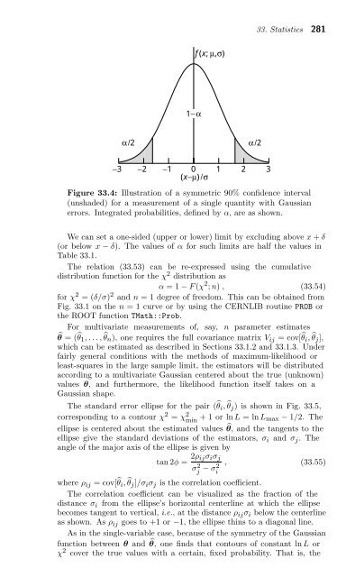
α/2<br />
1−α<br />
f (x; μ,σ)<br />
−3 −2 −1 0 1 2 3<br />
(x−μ)/σ<br />
33. Statistics 281<br />
α/2<br />
Figure 33.4: Illustration of a symmetric 90% confidence interval<br />
(unshaded) for a measurement of a single quantity with Gaussian<br />
errors. Integrated probabilities, defined by α, areasshown.<br />
We can set a one-sided (upper or lower) limit by excluding above x + δ<br />
(or below x − δ). The values of α for such limits are half the values in<br />
Table 33.1.<br />
The relation (33.53) can be re-expressed using the cumulative<br />
distribution function for the χ2 distribution as<br />
α =1− F (χ 2 ; n) , (33.54)<br />
for χ2 =(δ/σ) 2 and n = 1 degree of freedom. This can be obtained from<br />
Fig. 33.1 on the n = 1 curve or by using the CERNLIB routine PROB or<br />
the ROOT function TMath::Prob.<br />
For multivariate measurements of, say, n parameter estimates<br />
�θ =( � θ1,..., � θn), one requires the full covariance matrix Vij =cov[ � θi, � θj],<br />
which can be estimated as described in Sections 33.1.2 and 33.1.3. Under<br />
fairly general conditions with the methods of maximum-likelihood or<br />
least-squares in the large sample limit, the estimators will be distributed<br />
according to a multivariate Gaussian centered about the true (unknown)<br />
values θ, and furthermore, the likelihood function itself takes on a<br />
Gaussian shape.<br />
The standard error ellipse for the pair ( � θi, � θj) is shown in Fig. 33.5,<br />
corresponding to a contour χ2 = χ2 min +1 orlnL =lnLmax − 1/2. The<br />
ellipse is centered about the estimated values � θ, and the tangents to the<br />
ellipse give the standard deviations of the estimators, σi and σj. The<br />
angle of the major axis of the ellipse is given by<br />
tan 2φ = 2ρijσiσj<br />
σ2 j − σ2 , (33.55)<br />
i<br />
where ρij =cov[ � θi, � θj]/σiσj is the correlation coefficient.<br />
The correlation coefficient can be visualized as the fraction of the<br />
distance σi from the ellipse’s horizontal centerline at which the ellipse<br />
becomes tangent to vertical, i.e., at the distance ρijσi below the centerline<br />
as shown. As ρij goes to +1 or −1, the ellipse thins to a diagonal line.<br />
As in the single-variable case, because of the symmetry of the Gaussian<br />
function between θ and � θ, one finds that contours of constant ln L or<br />
χ2 cover the true values with a certain, fixed probability. That is, the