Particle Physics Booklet - Particle Data Group - Lawrence Berkeley ...

33. Statistics 283
νup = 1 −1
2 F
χ2 (1 − αup;2(n +1)), (33.59b)
where the upper and lower limits are at confidence levels of 1 − αlo and
1 − αup, respectively, and F −1
χ2 is the quantile of the χ2 distribution
(inverse of the cumulative distribution). The quantiles F −1
χ2 can be
obtained from standard tables or from the CERNLIB routine CHISIN. For
central confidence intervals at confidence level 1 − α, setαlo = αup = α/2.
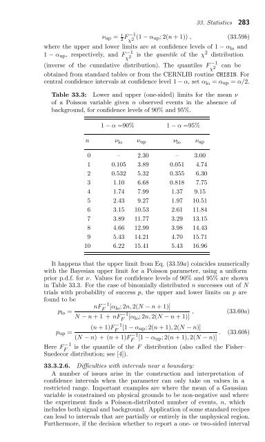
Table 33.3: Lower and upper (one-sided) limits for the mean ν
of a Poisson variable given n observed events in the absence of
background, for confidence levels of 90% and 95%.
1 − α =90% 1 − α =95%
n ν lo νup ν lo νup
0 – 2.30 – 3.00
1 0.105 3.89 0.051 4.74
2 0.532 5.32 0.355 6.30
3 1.10 6.68 0.818 7.75
4 1.74 7.99 1.37 9.15
5 2.43 9.27 1.97 10.51
6 3.15 10.53 2.61 11.84
7 3.89 11.77 3.29 13.15
8 4.66 12.99 3.98 14.43
9 5.43 14.21 4.70 15.71
10 6.22 15.41 5.43 16.96
It happens that the upper limit from Eq. (33.59a) coincides numerically
with the Bayesian upper limit for a Poisson parameter, using a uniform
prior p.d.f. for ν. Values for confidence levels of 90% and 95% are shown
in Table 33.3. For the case of binomially distributed n successes out of N
trials with probability of success p, the upper and lower limits on p are
found to be
nF
plo =
−1
F [αlo;2n, 2(N − n +1)]
N − n +1 + nF −1
F [α , (33.60a)
lo;2n, 2(N − n +1)]
(n +1)F
pup =
−1
F [1 − αup;2(n +1), 2(N − n)]
(N − n) +(n +1)F −1
F [1 − αup;2(n
. (33.60b)
+1), 2(N − n)]
Here F −1
F is the quantile of the F distribution (also called the Fisher–
Snedecor distribution; see [4]).
33.3.2.6. Difficulties with intervals near a boundary:
A number of issues arise in the construction and interpretation of
confidence intervals when the parameter can only take on values in a
restricted range. Important examples are where the mean of a Gaussian
variable is constrained on physical grounds to be non-negative and where
the experiment finds a Poisson-distributed number of events, n, which
includes both signal and background. Application of some standard recipes
can lead to intervals that are partially or entirely in the unphysical region.
Furthermore, if the decision whether to report a one- or two-sided interval