Codes sur des anneaux nis et r eseaux arithm ... - Alexis Bonnecaze

THESE
de doctorat de
L'Universite de Nice - Sophia Antipolis
et de
L'Ecole doctorale Sciences Pour l'Ingenieur
Pour obtenir le titre de
Docteur en Sciences
Specialite : Informatique
Presentee par
Alexis BONNECAZE
Codes sur des anneaux nis et reseaux
Composition du Jury :
arithmetiques
Soutenue le 10 novembre 1995
M. Jacques Wolfmann President
Mme Christine Bachoc Rapporteur
M. Robert Calderbank Rapporteur
M. Claude Carlet Rapporteur
Mme Claudine Peyrat Examinateur
M. Bernard Mourrain Examinateur
M. Patrick Sole Directeur
These preparee a l'Universite de Nice - Sophia Antipolis, Laboratoire
Informatique Signaux et Systemes de Sophia Antipolis, C.N.R.S. - U.R.A. 1376

3
Amesparents

Remerciements
Je voudrais exprimer toute ma reconnaissance aux membres du jury,
a Jacques WOLFMANN qui a eu la gentillesse de nous inviter, Pierre Loyer et moi, a
participer aux seminaires du GECT, et qui a bien voulu presider le jury,
a Christine BACHOC et Claude CARLET qui ont accepte la lourde charge de rapporteur,
et dont les discussions me furent precieuses,
a Claudine PEYRAT qui a consacre du temps aussi bien pour m'aider dans des taches
administratives que pour me donner des conseils dans la redaction de la these,
a Bernard MOURRAIN qui a su me faire partager ses connaissances dans le domaine
de la theorie des invariants,
aPatrick SOLE qui m'a initie aux joies de la theorie des codes. Il a su me faire partager
la passion scienti que qui l'anime et m'a permis de conna^tre le monde exaltant dela
recherche.
Avec Patrick Sole, quatre personnes ont joueunr^ole essentiel dans l'accomplissement
de cette these,
Robert CALDERBANK, qui m'a fait l'honneur de m'accueillir aux \Bell Labs" en janvier
94. Son experience de la recherche et ses connaissances immenses demeurent pour
moi exemplaires,
Vijay KUMAR, qui a eu la gentillesse de m'inviter un an a USC. Ce fut une experience
tres enrichissante. J'ai beaucoup apprecie sa simplicite et sa maniere de travailler, tres
decontractee mais terriblement e cace. J'en pro te pour remercier tous les membres du
labo EE de USC et en particulier Dr Irving REED et Xuemin CHEN, Abhijit SHANB-
HAG, Milly MONTENEGRO etJohnFOSTER pour leur aide et soutien, ainsi que
Robert GURALNICK, Chairman du departement de mathematiques aUSC.
Iwan DUURSMA qui m'a fait decouvrir un autre visage de l'algebre. Ses discussions
m'ont enormement apporte. Je lui dois beaucoup,
Jean-Claude BERMOND, qui a accepte de m'accueillir dans son laboratoire, et m'a permis
d'e ectuer le stage aUSC.
En n, je remercie tous les membres du labo I3S qui m'ont aideetsoutenu, et plus particulierement
Pierre LOYER qui fut d'un soutien constant etdont j'ai apprecie leserieux
et les qualites pedagogiques, ainsi que Danielle GERIN et Patricia LACHAUME pour
leur aide administrative.
5

Table des matieres
1 Preliminaires mathematiques 15
1.1 Les anneaux de Galois :::::::::::::::::::::::::::: 15
1.1.1 De nitions et proprietes fondamentales : : : : : : : : : : : : : : : 15
1.1.2 Parametres d'un anneau de Galois R :::::::::::::::: 17
1.1.3 Extensions de l'anneau de Galois R::::::::::::::::: 17
1.1.4 Les inversibles de GR(p n m) ::::::::::::::::::::: 20
1.1.5 L'anneau de Galois R = GR(4m) :::::::::::::::::: 20
1.1.6 Le relevement de Hensel ::::::::::::::::::::::: 23
1.1.7 L'application trace :::::::::::::::::::::::::: 23
1.2 Le code de Golay binaire ::::::::::::::::::::::::::: 24
1.2.1 Combinatoire ::::::::::::::::::::::::::::: 25
1.2.2 Le code de Golay binaire ::::::::::::::::::::::: 26
1.2.3 Le MOG :::::::::::::::::::::::::::::::: 29
1.3 Theorie des invariants :::::::::::::::::::::::::::: 33
1.3.1 Theorie des invariants :::::::::::::::::::::::: 33
1.3.2 Le package Invar de Maple et le logiciel Macaulay : : : : : : : : : 35
2 Codes quaternaires 37
2.1 Notions de base :::::::::::::::::::::::::::::::: 37
2.1.1 Enumerateurs de poids :::::::::::::::::::::::: 39
2.1.2 Identite de MacWilliams ::::::::::::::::::::::: 40
2.2 L'application Gray-map ::::::::::::::::::::::::::: 42
2.2.1 Proprietes de l'application Gray-map :::::::::::::::: 43
2.2.2 Conditions de linearite et d'auto-dualite :::::::::::::: 44
2.3 Dualite formelle et Z 4-dualite : : : : : : : : : : : : : : : : : : : : : : : : 47
2.4 Constructions de codes quaternaires ::::::::::::::::::::: 48
2.5 Relevements de Hensel de codes binaires :::::::::::::::::: 49
2.6 Idempotents des codes cycliques quaternaires :::::::::::::::: 51
3 Translates des codes quaternaires 53
3.1 Codes de Kerdock, Nordstrom-Robinson, et Preparata :::::::::: 53
3.1.1 Le code de Kerdock :::::::::::::::::::::::::: 54
3.1.2 Le code de Nordstrom-Robinson ::::::::::::::::::: 55
3.1.3 Le code de Preparata ::::::::::::::::::::::::: 55
3.2 Translates of Linear Codes over Z 4 : : : : : : : : : : : : : : : : : : : : : 56
7

8 TABLE DES MATIERES
3.2.1 Introduction :::::::::::::::::::::::::::::: 56
3.2.2 Linear Codes over Z 4 ::::::::::::::::::::::::: 57
3.2.3 Galois Rings over Z 4 ::::::::::::::::::::::::: 60
3.2.4 Families of Codes ::::::::::::::::::::::::::: 63
3.2.5 Translates of Linear Codes :::::::::::::::::::::: 68
3.2.6 Punctured Preparata Codes ::::::::::::::::::::: 70
3.2.7 Preparata Codes ::::::::::::::::::::::::::: 74
3.2.8 Codes of small length ::::::::::::::::::::::::: 76
3.2.9 Lee metric ::::::::::::::::::::::::::::::: 79
3.2.10 Conclusions :::::::::::::::::::::::::::::: 82
4 Codes residus quadratiques quaternaires 83
4.1 Construction de R. Calderbank ::::::::::::::::::::::: 83
4.2 Construction standard :::::::::::::::::::::::::::: 87
4.3 Idempotents des codes residus quadratiques :::::::::::::::: 87
4.4 Proprietes sur les poids euclidiens :::::::::::::::::::::: 89
4.5 Exemples de codes residus quadratiques quaternaires : : : : : : : : : : : 89
4.5.1 Le Golay quaternaire ::::::::::::::::::::::::: 89
4.5.2 Autres exemples de Codes residus quadratiques quaternaires ::: 94
4.6 Connexion avec la transformee de Fourier :::::::::::::::::: 95
4.7 Borne en racine carree de poids minimum :::::::::::::::::: 95
5 Codes de type II 97
5.1 Codes auto-duaux ::::::::::::::::::::::::::::::: 97
5.2 Codes de type II ::::::::::::::::::::::::::::::: 98
5.2.1 Exemples de codes de type II ::::::::::::::::::::100
5.2.2 Codes quaternaires doublement circulants : : : : : : : : : : : : :103
6 Reseaux unimodulaires 105
6.1 Quatre constructions quaternaires pour le reseau de Gosset E 8 ::::::107
6.2 Le reseau de Leech ::::::::::::::::::::::::::::::108
6.3 Le reseau de Barnes-Wall BW 32 :::::::::::::::::::::::110
6.4 Le reseau BSBM 32 ::::::::::::::::::::::::::::::110
6.5 Une table de codes et reseaux ::::::::::::::::::::::::111
A Enumerateurs de poids complets des polyn^omes de base 115

Preface
La these decrit les resultats de mes recherches sur les codes quaternaires. Mon travail
de recherche s'est e ectue en partie a l'I3S (Sophia-Antipolis), et a USC (Los Angeles)
dans le departement Electrical Engineering sous la direction du professeur P.V. Kumar.
Il a fait l'objet de quatre articles:
1. Avec P. Sole
Quaternary Constructions of Formally Self-Dual Binary Codes and Unimodular
Lattices"
First French-Israeli Workshop on Algebraic Coding, Springer Verlag, 1994.
2. Avec P. Sole et R. Calderbank
Quaternary Quadratic Residue Codes and Unimodular Lattices
IEEE Transactions on information theory, March, Vol 41, N0. 2,1995.
3. Avec P. Sole, C. Bachoc et B. Mourrain
Quaternary Type II codes
Soumis a IEEE Transactions on information theory.
4. Avec I. Duursma
Translates of Z 4-linear Codes
Soumis a IEEE Transactions on information theory.
Le premier article peut ^etre considere comme une version preliminaire du deuxieme article.
Nous avons etudie principalement les codes residus quadratiques quaternaires et
la construction de reseaux unimodulaires pairs a partir de codes quaternaires. Le reseau
de Leech peut^etre determine de cette maniere. L'article (3) traite des codes de type II.
Ils sont caracterises par leurs proprietes sur les enumerateurs de poids. Une construction
d'un reseau pair unimodulaire en dimension 32 est donnee. Le quatrieme article decrit
une methode permettant dedeterminer les cosets des codes quaternaires.
Ces quatre articles forment l'ossature de la these. L'introduction developpe plus en
detail son plan general ainsi que les contributions qu'elle amene.
9

10 TABLE DES MATIERES

Introduction
En 1623, Francis Bacon constatait qu'un homme pouvait s'exprimer a distance au moyen
de signes binaires. Mais il fallut attendre 1948, et les publications de Claude Shannon,
pour que s'etablisse une theorie des communications numeriques rigoureuse. Cette
theorie, connue sous le nom de theorie de l'information, t dispara^tre les \bricolages
astucieux" aux idees quelquefois preconcues pour laisser place adevraiestechniques
scienti ques.
Un des problemes majeurs que Shannon (voir [Sha49]) etudia est la garantie d'une
communication able en presence de bruit. Ce probleme est intimement liea la notion
de codage. Cependant, la theorie se contente de predire l'existence de codes et ne donne
aucun moyen de les construire. Depuis les annees cinquante, des progres considerables
ont ete e ectues en matiere de conception de systemes de communications numeriques,
mais le probleme de la construction de \bons codes" reste toujours d'actualite.
La problematique du codage correcteur est simple: on desire proteger un message
contre les erreurs. Un message est compose d'une suite d'elements appartenant aunensemble
ni (ou alphabet) appeles symboles d'information. L'alphabet est le plus souvent
binaire. Lors de la transmission d'un message, il arrive occasionnellement que surviennent
des erreurs. Celles-ci peuvent ^etre la consequence de bruit sur le canal et peuvent
grandement a ecter la qualite de la transmission. Pour prevenir ce risque, on adjoint
aunblocdek symboles d'information (le message a transmettre) un certain nombre
de symboles calcules en fonction du message par l'intermediaire d'une fonction xee
a l'avance. Cela revient a ajouter une redondance au message a transmettre. Cette
concatenation des k symboles d'information avec la redondance represente un \mot de
code" x de longueur N>k. L'ensemble de tous les mots obtenus de cette facon forme
un \code en bloc" de longueur N. Connaissant la fonction , il est facile de veri er
l'appartenance d'un mot au code et de detecter une erreur eventuelle. Un \bon code"
doit compter un grand nombredemotstres distincts les uns des autres. Il doit donc
permettre d'envoyer des messages tres varies et de reduire la possibilite de confusion
entre les mots.
La plupart du temps, et pour des raisons pratiques, on utilise des codes lineaires.
Concretement, un code lineaire de longueur N sur un corps ni F est un sous groupe
additif de F N . Ces codes permettent detravailler sur des matrices plut^ot que sur des
ensembles. Ils sont donc plus faciles aetudier, a coder et adecoder. Cependant, la
linearite induit une structure qui limite quelquefois la cardinalite du code. Lorsque l'on
desire maximaliser le nombre de mots du code possible, avec une longueur et une capacite
de correction donnees, il est souvent necessaire de considerer des codes non lineaires. Les
11

12 TABLE DES MATIERES
exemples les plus celebres de codes non lineaires sont les codes de Preparata, Kerdock et
Nordstrom-Robinson. Les codes de Preparata et Nordstrom-Robinson contiennent par
exemple deux fois plus de mots que les meilleurs codes lineaires de m^eme parametres.
Les codes de Preparata et Kerdock sont d'une certaine maniere \duaux" l'un de
l'autre, bien que leur absence de linearite ne permette pas de parler de dualitealgebrique.
La propriete qui les fait ressembler a des codes duaux s'exprime sur leur enumerateur de
distances: l'image de l'enumerateur de l'un par la transformation de MacWilliams donne
l'enumerateur de l'autre. Cette propriete est toujours vraie pour des codes lineaires,
duaux l'un de l'autre. Dans [Cam79], P. Camion pose la question de savoir si cette
dualite formelle vient d'une dualite plus forte qui reste ade nir.
En 1992, Hammons et al. [HKC + 94] donnerent une explication de cette dualite formelle
en de nissant les codes de Kerdock et Preparata sur l'anneau Z 4 des entiers modulo
quatre. Sur cet anneau, ces codes sont lineaires et algebriquement duaux. L'application
\Gray map", qui permet de passer de la representation quaternaire a la representation
binaire est extr^emement simple. Elle joue un r^ole fondamental dans le developpementde
l'etude des codes quaternaires. C'est une isometrie qui preserve la propriete de distance
invariante mais non la linearite. Les nouvelles de nitions des codes de KerdocketPreparata
sont tres naturelles: ce sont des codes cycliques etendus sur Z 4.Plusgeneralement,
les decouvertes de Hammons et al. donnent une methode pour construire de nouveaux
codes binaires non lineaires. Elles permettent aussi de construire des codes binaires
formellement auto-duaux, images par la \Gray-map" de codes auto-duaux sur Z 4. Les
codes binaires formellement auto-duaux sont interessants car ils admettent souvent de
tres bons parametres.
Un autre aspect interessant des codes quaternaires consiste en leurs liens avec les
reseaux arithmetiques. Ce sujet n'a pas encore eteetudiedemaniere exhaustive. Cependant,
des constructions tres simples utilisant des codes sur Z 4 permettent dedeterminer
certains reseaux celebres. Les constructions du reseau de Gosset E 8,dureseau de Leech
24 et du reseau de Barnes-Wall BW 32 en sont quelques exemples.
Dans cette these, nous abordons les di erents aspects des codes lineaires sur Z 4.
Nous nous interessons aux proprietes des codes quaternaires, aladetermination de leurs
translates, puis a certaines constructions de reseaux arithmetiques. Nous utilisons pour
cela plusieurs theories dont les bases sont presentees au chapitre 1. Ce chapitre peut
^etre considere comme une etude bibliographique.
Dans le chapitre 2, nous rappelons les de nitions et proprietes les plus utiles concernant
les codes lineaires sur Z 4 que nous appelons codes quaternaires. Un grand nombre
de ces resultats ont ete publies dans [HKC + 94]. Nous introduisons en particulier l'application
\Gray-map" et evoquons la Z 4-linearite etZ 4-dualite que C. Carlet etudie en
detail dans [Car].
La construction du code de Kerdock Z 4-lineaire de Hammons et al. dans [HKC + 94]
utilise le relevement de Hensel (aussi appele lift de Hensel) d'un code cyclique binaire
pour obtenir un code cyclique sur Z 4. Le relevement de Hensel est une procedure
algebrique qui associe aunpolyn^ome binaire un unique polyn^ome a coe cients dans Z 4.

TABLE DES MATIERES 13
L'utilisation de relevements successifs produit un code sur Z 2 a (a >1) et un code de ni
sur les entiers 2-adiques, Z 2 1, que R. Calderbank nomme \code universel". Les codes
de nis sur Z 2 a peuvent ^etre obtenus a partir du code universel par reduction modulo
2 a . L'etude des codes cycliques binaires et quaternaires peut aider a la comprehension
des codes universels. Cependant, les codes quaternaires sont d'un inter^et considerable
en eux-m^eme. Nous etudions leurs idempotents et, dans le chapitre 3, decrivons une
methode permettant dedeterminer les enumerateurs de poids complets des classes
laterales de ces codes. Nous adaptons au cas quaternaire le travail de P. Camion dans
[CCD92] et travaillons sur des partitions regulieres. Nous montrons que le code de Hamming
quaternaire etendu admet dix classes laterales d'enumerateurs de poids complets
distincts.
Les codes residus quadratiques binaires representent une famille de codes cycliques
des plus interessantes. Determiner la capacite de correction d'erreurs asymptotique de
ces codes est enonce comme un probleme de recherche dans le livre de MacWilliams et
Sloane [MS77] et n'a toujours pas ete resolu. Nous examinons en detail les \releves" de
ces codes, les residus quadratiques quaternaires. Nous construisons leurs idempotents,
proposons une borne en racine carree sur le poids de Lee minimum et etudions la relation
avec la transformee de Fourier nie. L'exemple le plus interessant de ces codes est le
relevement de Hensel du code de Golay que l'on nomme le Golay quaternaire. Tout
comme le code de Golay binaire, il possede des \designs". Il fait partie de la famille des
codes de type II que nous de nissons au chapitre 5.
Les codes de typeIIsont des codes auto-duaux dont tous les poids euclidiens sont
des multiples de 8. Nous caracterisons leurs enumerateurs de poids en utilisantlatheorie
des invariants. Nous determinons de cette facon les enumerateurs de poids des codes
residus quadratiques quaternaires en longueur 32 et 48.
Le chapitre 6 decrit une methode permettant de construire des reseaux unimodulaires
pairs a partir de codes auto-duaux sur Z 4. La classe des reseaux unimodulaires
pairs inclut le reseau de Gosset E 8 et le reseau de Leech 24. Nos constructions de
reseaux utilisent une construction A adaptee au cas quaternaire. Un code quaternaire C
determine un reseau (C) qui consiste en tous les vecteurs acoe cients entiers qui sont
congrus a un mot de code modulo 4. Nous prouvons que si C est un code de type II,
(C)=2 est un reseau pair et unimodulaire. Nous montrons que quand q = ;1 (mod 8)
est une puissance d'un nombre premier, les codes residus quadratiques etendus quaternaires
satisfont cette condition. C'est le cas du code de Golay quaternaire qui permet de
determiner le reseau de Leech 24 de cette facon. Cette construction appara^t comme la
plus simple connue acejourdececelebre reseau.

14 TABLE DES MATIERES

Chapitre 1
Preliminaires mathematiques
L'objet de ce chapitre est de presenter certains outils ou notions de base (les anneaux de
Galois, le code de Golay binaire, et la theorie des invariants) qui seront utilises dans les
chapitres suivants. Il s'agit donc avant tout de donner, ou rappeler, quelques de nitions
et proprietes permettant une comprehension plus aisee de la these.
1.1 Les anneaux de Galois
Il semble que ce soit Krull qui en 1923 [Kru23] ait etudie etdeveloppe pour la premiere
fois les anneaux de Galois, puis en 1979, Shankar [Sha79] qui les ait utilises en theorie
des codes dans le cadre d'etudes sur les codes BCH sur des anneaux. Nous allons voir
qu'il existe une analogie profonde entre les anneaux et les corps de Galois. Ainsi, le r^ole
joue par les anneaux de Galois est souvent similaire a celui joue par les corps de Galois
dans la theorie traditionnelle, les problemes centraux etant toujours des problemes de
divisibilite et de factorisation de polyn^omes.
Nous etudions ici les anneaux de Galois et les extensions galoisiennes dont les proprietes
seront utiles lors des constructions des codes. Nous ne considerons que des anneaux nis.
Un expose plus detaille sur l'etude des anneaux nis peut ^etre trouve dans [McD74b],
[Lan80] et certaines autres proprietes dans [Nec91].
Nous rappelons dans un premier temps quelques de nitions et proprietes elementaires.
1.1.1 De nitions et proprietes fondamentales
Dans toute la suite, R represente un anneau ni.
Notons l'element neutre multiplicatif 1.
Un diviseur de zero de R est un element x \qui divise" zero, c'est a dire pour qui il existe
y 6= 0 dans R tel que xy =0. Uninversible de R est un element X de R qui \divise 1".
En d'autres termes, on a xy = 1 pour un certain y dans R. L'element y est alors note x ;1 .
De nition 1.1 R est un anneau de Galois s'il est commutatif, unitaire, et si l'ensemble
de tous les diviseurs de zero est de la forme pR, p etant un entier premier.
15

16 CHAPITRE 1. PRELIMINAIRES MATHEMATIQUES
Les corps de Galois peuvent donc^etre consideres comme des anneaux de Galois ne
contenant pas de diviseurs de zero. L'exemple le plus utilise entheorie de codes est
R = Zp n, l'anneau des entiers modulo pn .
La caracteristique char R de R est l'ordre additif du neutre multiplicatif, 1.
Ainsi (Zn +:) est un anneau de caracteristique n, puisque 1 est d'ordre n dans (Zn +):
La caracteristique d'un anneau R de Galois est
char R = p n n2 N:
Un anneau est integre s'il est non nul et sans diviseur de zero.
Un ideal I de R est dit maximal si I 6= R et s'il n'existe aucun ideal propre contenant
I. SiR est un anneau et I un ideal maximal, alors R=I est un corps.
Un anneau est dit local s'il admet un unique ideal maximal. Ainsi les assertions suivantes
sont equivalentes:
1. R est un anneau local.
2. R admet exactement unideal maximal.
3. Les diviseurs de zero de R sont contenus dans un ideal propre.
4. Les diviseurs de zero de R forment unideal.
5. Les diviseurs de zero de R forment un groupe commutatif additif.
6. Pour tout x dans R, un des 2 elements de l'ensemble fx 1+xg estuninversible.
Exemple: Les anneaux Z 4 (Z 2) (Z 2) Z 2[X]=(X 2 +1) Z 2[X]=(X 2 + X +1)sont les
seuls anneaux de 4 elements.
Z 4 est isomorphe a Z 2[X]=(X 2 ) et a pour ideal maximal I = f0 2g =2R. C'est
un anneau de Galois.
(Z 2) (Z 2) admet comme ideaux les trois ensembles constitues de (0 0) et d'un
element nonnul. Son seul element inversible est (1 1).
Z 2[X]=(X 2 +1)apourideal maximal I = f0 X +1g. Ses elements inversibles
sont 1etX.
Z 2[X]=(X 2 + X + 1) est le corps a quatre elements F 4.
Nous allons voir que d'une maniere generale, l'anneau Zp n est un anneau local pour n
premier. C'est de plus un anneau de Galois.

1.1. LES ANNEAUX DE GALOIS 17
1.1.2 Parametres d'un anneau de Galois R
A partir de maintenant et jusqu'a la nduchapitre, R represente un anneau de Galois
de caracteristique p n et D = pR l'ensemble des diviseurs de zero de R.
Notons \n" lesymbole representant la soustraction ensembliste. Le groupe multiplicatif
R ? de l'anneau est
R ? = R n pR = R n D
puisque les diviseurs de zero sont lesseulselements non inversibles dans un anneau ni.
Les elements de R ? sont donclesinversibles de R et D est l'unique ideal maximal de R.
De plus l'anneau
R = R=D
est le corps de Galois GF (q) (q etant une puissance de p, p r ). Notons 1l'element neutre
de R. Nous avons donc 1=1+D:
Posons D t = p t R et t 2f0::: n; 1g. On a alors
D n;1 6=0 et D n =0
Et la chaine suivante d'ideaux admet des inclusions strictes:
R = D 0 D = pR :::D n;1 = p n;1 R D n = p n R =0:
Tout comme la caracteristique, le cardinal de l'anneau est importantpourladetermination
de R. Nous verrons que ces deux parametres determinent completement, a isomorphisme
pres, l'anneau de Galois. Nous allons prouver que le nombre d'elements de l'anneau R
et du groupe multiplicatif R ? sont
jRj = q n jR ? j =(q ; 1)q n;1 :
Il su t pour cela de prouver que pour chaque t 2f0::: n; 1g nous avons l'egalite
jp t R=p t+1 Rj = q: Posons Rt = p t R=p t+1 R. R est visiblement un espace vectoriel sur
R = GF (q). De plus dim R Rt = 1. En e et considerons 2 p t R n p t+1 R,nousavons
R = p t R et R = Rt: Ainsi, jRj = q n et le cardinal de R ? decoule immediatement.
1.1.3 Extensions de l'anneau de Galois R
R = R=pR est appele corps de classe residuelle de l'anneau de Galois R de caracteristique
p n . Ilexisteunepimorphisme d'anneau naturel R ! R qui peut s'etendre en epimorphisme
d'anneau des polyn^omes
R[X] ! R[X] R[X]=pR[X]:
Soit A(X) = P aiX i 2 R[X] un polyn^ome. Son image par l'epimorphisme est
A(X) = X aiX i 2 R[X]:
Un b-polyn^ome (basic irreducible polynomial en anglais) f(X) 2 R[X] sur R est un
polyn^ome unitaire tel que f(X) est un polyn^ome irreductible sur le corps R: Nous allons

18 CHAPITRE 1. PRELIMINAIRES MATHEMATIQUES
montrer que la donnee d'un b-polyn^ome f de degre m sur R permet de construire un
plus gros anneau en adjoignant a R une racine de f. Nous appelons cette extension une
G-extension de R. Le b-polyn^ome f(X) 2 R[X] permet de considerer la G-extension
S = R[X]=(f(X)). Montrons que S est un anneau de Galois.
Theoreme 1.1 Soit R un anneau de Galois de q n elements et de caracteristique p n .
Soit f(X) un b-polyn^ome sur R de degre m. Alors l'anneau
S = R[X]=(f(X))
estunanneau de Galois de parametres char S = p n jSj = q mn .
Preuve. Si le calcul des parametres de l'anneau ne pose aucune di culte, il convient
de prouver que S est un anneau de Galois. Trivialement, les elements de pS sont des
diviseurs de zero. Il faut donc veri er que tous les elements de SnpS sont desinversibles.
Considerons un element deS n pS. Il peut s'ecrire de facon unique
=[A(X)]f = A(X)+f(X)R[X]
ou A(X) 2 R[X] degA(X)

1.1. LES ANNEAUX DE GALOIS 19
Exemple:
Soit R 8 = Z 2 3 = Z 8 l'anneau des entiers modulo 8.
Posons S 8 = R[X]=(f(X)) avec f(X) =X 3 +6X 2 +5X +7.
Le polyn^ome f est un b-polyn^ome et f(X) =X 3 + X +1.
L'ensemble des diviseurs de zero de S est D 8 =2S 8 de cardinal jD 8j =4 3 et le cardinal
des elements inversibles est jS ? 8j =8 3 ; 4 3 =(2 3 ; 1)4 3 .
L'anneau S 8 est une G-extension de degre 3deR 8.
En regle generale, si l'on considere un element de S, le sous anneau
fA( ):A(X) 2 R[X]g
de R est note R[ ]. C'est une extension de l'anneau R par . Dans l'exempleprecedent,
S 8 = R 8[ ]ou est une racine de f(X). L'anneau S 8 peut donc s'ecrire en tant que
module < 1 2 >.
Le prochain theoreme montre le lien profond qui existe entre le corps et l'anneau de
Galois. Sa preuve utilise le lemme suivant qui lie une racine d'un polyn^ome A(X) de
R[X] a une racine du polyn^ome residuel A(X) dansR:
Lemme 1.3 Soient A(X) 2 R[X] et 2 S tels que A( )=0 et A 0 ( ) 6= 0. Alors il
existe une unique racine 2 S du polyn^ome A(X) telle que = :
Preuve. Voir [Nec91]. 2
Theoreme 1.2 Soit S une G-extension de degre m de R et f(X) un b-polyn^ome sur R
de degre k. Alors
1. Le polyn^ome f(X) auneracine dans S si et seulement si kjm.
2. Si kjm, f(X) admet exactement k racines distinctes 1::: k dans S modulo
l'ideal pS f(X) =(X ; 1) :::(X ; k).
3. Pour tout element 2 S, onaS = R[ ] si et seulement si est une racine du
b-polyn^ome de degre m sur R.
Preuve. Voir [Nec91]. 2
Un corollaire important decetheoreme est:
Corollaire 1.1 Soit S un anneau de Galois de caracteristique p n et de cardinalite p mn ,
alors
S Zp n[X]=(f(X))
ou f(X) est un b-polyn^ome de degre m sur Zp n. Notons un tel anneau GR(pn m):
Ainsi, deux anneaux de Galois sont isomorphes si et seulement si ils ontm^eme cardinalite
et caracteristique.
Remarque. GR(pn 1) = Zp n et GR(p m) =Fpm .
Une consequence du lemme 1.3 est:
Corollaire 1.2 Soit a un entier impair, alors X a ; 1 admet une factorisation unique
dans S.

20 CHAPITRE 1. PRELIMINAIRES MATHEMATIQUES
1.1.4 Les inversibles de GR(p n m)
Theoreme 1.3 Soit S = GR(p n m). Legroupe multiplicatif des inversibles de S peut
s'ecrire comme le produit direct de deux groupes:
ou
S ? = G 1
1. G 1 est un groupe cyclique d'ordre p m ; 1
2. G 2 est un groupe d'ordre p (n;1)m tel que
(a) Si p est impair, ou si p =2et n 2, alors G 2 est un produit direct de m
groupes cycliques chacun d'ordre p n;1
(b) Si p =2et n 3, alors G 2 est un produit direct d'un groupe cyclique d'ordre
2, ungroupe cyclique d'ordre 2 n;2 et m ; 1 groupes cyclique chacun d'ordre
2 n;1
Preuve. Voir [McD74b]. 2
Reprenons l'exemple precedent: R = Z 8 et S 8 = R[X]=(f(X)) avec
G 2
f(X) =X 3 +6X 2 +5X +7:
Alors f(X) divise X 7 ; 1dansZ 8[X]. Soit une racine primitive def(X), l'ordre de
est 2 3 ; 1 = 7. Notons H le groupe cyclique engendre par et K le corps residuel de
S, il vient
H (K ):
Soit U =1+2S 8 +4S 8,ona(U ) (S 4 +) ou S 4 Z 4=(f(X) mod 4). Ainsi
S ? 8 (K ) (S 4 +):
Il s'ensuit que l'ordre multiplicatif maximal d'un element deS ? 8 est 4(2 m ; 1) = 28.
1.1.5 L'anneau de Galois R = GR(4m)
Nous avons vu que l'anneau Z 4 = f0 1 2 3g des entiers modulo 4 est local. Son
unique ideal maximal, 2Z 4 = f0 2g est compose des diviseurs de zero. Soit f 2 Z 4[X],
nous de nissons l'application projection comme etant l'application : Z 4[X] !
GF (2)[X] qui reduit modulo 2 les coe cients de f(X) 2 Z 4[X]. Ainsi, un b-polyn^ome
f 2 Z 4[X] est un polyn^ome unitaire tel que (f) est irreductible sur Z 2.
Lemme 1.4 Le polyn^ome X a ; 1 (a impair et strictement positif) admet une factorisation
unique sur Z 4[X]. Cette factorisation etablit une correspondance biunivoque avec
la factorisation sur Z 2.

1.1. LES ANNEAUX DE GALOIS 21
Preuve. Voir le theoreme 1.2 et corollaire 1.2. 2
Les facteurs qui divisent Xa ; 1 mais pas Xa0 ; 1 pour a>a0 sont appeles des facteurs
primitifs. Considerons un polyn^ome h 2, de degre m, a coe cients binaires, qui soit un
facteur primitif de X a ; 1(a impair). Alors il existe un polyn^ome unitaire h 2 Z 4[X] de
degre m tel que h 2(X) = (h(X)) et h(X) diviseX a ; 1(mod4).
De nition 1.2 Soit f un b-polyn^ome de degre m sur Z 4. L'anneau de Galois R =
GR(4m) est de ni a un isomorphisme pres comme etant Z 4[X]=(f):
Soit une racine primitive def(X) etf(X) un facteur primitif de X 2m ;1 ; 1. Alors,
l'anneau de Galois R = GR(4m)peut^etre de ni comme etant l'extension R = Z 4[ ].
L'anneau R est d'ordre 4 m . Les diviseurs de zero forment un sous groupe, 2R, d'ordre
2 m . Le groupe des inversibles R ? = R n 2R qui est d'ordre (2 m ; 1)2 m , est un produit
direct de 2 groupes G 1 et G 2. D'apres le theoreme 1.3, Le sous groupe G 1 est un groupe
cyclique d'ordre a, que l'on va noter T ? car il est souvent appele systeme de Teichmuller
lorsqu'on lui adjoint 0. On pose alors T = T ? [f0g. L'ensemble
T = f0 1
2 :::
2 m ;2 g
peut ^etre decrit comme l'ensemble des zeros dans R de l'equation X 2m ;X. Notons que,
contrairement a R=2R, T n'a pas la structure d'un corps de Galois GF (2m).
Les elements de R admettent une representation unique `multiplicative' ou `additive'.
Dans la premiere representation, que l'on appelle aussi 2-adique, un element c 2 R s'ecrit
c = a +2b ou a et b appartiennent a T .
Lemme 1.5 Tout element de R admet une ecriture unique sous la forme c = a +2b ou
a et b appartiennent a T:
Preuve. La cardinalite deT est 2m ; 1. De plus, considerons deux ecritures di erentes
de c: c = a1 +2b1 et c = a2 +2b2: En elevant au carre les deux membres de l'egalite, on
obtient a2 1 = a2 2, eta1 = a2 pour a1a22 T . Il s'en suit que b1 = b2. 2
Soit l'application : c 7! a. Lenoyau de est le groupe G2 des elements de la forme
1+2b, ou b 2 T . Ainsi,
(c) =c 2m
c 2 R:
Remarque. On en deduit facilement (car c2m l'ensemble des carres dans l'anneau R.
L'application satisfait les equations [Yam90]
=(c2r;1) 2 ) que l'ensemble T represente
(cd) = (c) (d) et (c + d) = (c) (d)+2(cd) 2m;1
:
Un resultat classique de Paley et Todd dit que l'ensemble descarres dans un corps de
Galois de taille q =4n ; 1 forme un ensemble de di erences. Chaque inversible dans le
corps peut s'ecrire de n facons distinctes comme la di erence de deux carres (n;1 facons
pour la di erences de deux carres non nuls). Le lemme precedent montre que pour un
anneau de Galois R = GR(4m), un diviseur de zeronepeutpass'ecrire comme la
di erence de deux carres. Le prochain lemme montre que tout inversible dans l'anneau
s'ecrit d'une maniere unique comme di erence de deux carres. Les preuves du lemme et
theoreme suivants sont presentees au chapitre 3 dans la section \Galois rings over Z 4".

22 CHAPITRE 1. PRELIMINAIRES MATHEMATIQUES
Lemme 1.6 Dans l'anneau R = GR(4m), l'ensemble des solutions (x y a b), tel que
x y a b 2 T ,coincide pour l'equation
et le systeme d'equations
a +2b = x ; y (1.1)
a 2 +2ab + b 2 = xa (1.2)
b 2 = ya (1.3)
x = y si a =0: (1.4)
Theoreme 1.4 Soit R = GR(4m)m>0, et soit T l'ensemble des carres de R.
(a) L'ensemble T +2T =(x+2y : x y 2 T ) contient chaque element de R avec comme
multiplicite 1.
(b) L'ensemble T ; T =(x ; y : x y 2 T ) contient 0 avec une multiplicite 2 m , aucun
autre diviseur de zero, et les inversibles avec une multiplicite de1.
(c) L'ensemble T + T =(x + y : x y 2 T ) contient les diviseurs de zero avec une
multiplicite de1, et la moitie des inversibles avec multiplicite deux.
(d) Les ensembles T +T and ;(T +T ) coincident lorsque m est pair. Si m est impair,
ils s'intersectent en 2R.
Remarque. Ce resultat a un inter^et combinatoire. Il permet en e et de construire des
di erences d'ensembles (des PDS et RDS, \perfect di erence set" et \relative di erence
set" respectivement) a partir de l'anneau de Galois R.
Les elements de l'anneau peuvent aussis'ecrire dans une autre representation que
l'on appelle additive. Dans cette representation, un element c 2 R s'ecrit
c =
m;1 X
r=0
br
r
br 2 Z 4:
Il est facile de voir que cette ecriture est unique. Elle donne 4 m elements di erents.
Intuitivement elle permet de mieux comprendre la notation Z 4[ ]: il s'agit de tous les
polyn^omes en a coe cients dans Z 4, modulo le polyn^ome minimal de :
Exemple: Reprenons l'exemple precedent avec h(X) =X 3 +2X 2 + X ; 1et une
racine de h: Alors
3 = 2 2 +3 +1
4 = 3 2 +3 +2
5 = 2 +3 +3
6 = 2 +2 +1
7 = 1
Ainsi, l'element c =1+3 5 s'ecrit dans la representation additive 2+ +3 2 :
c = 1+3 5
1 + 3(3 + 3 + 2 )
1+1+ +3 2
2+ +3 2 :

1.1. LES ANNEAUX DE GALOIS 23
1.1.6 Le relevement de Hensel
Considerons un polyn^ome h 2(X) 2 Z 2[X] de degre m, qui soit un facteur primitif de
x a ; 1 (a impair): Alors, nous savons qu'il existe un unique polyn^ome unitaire h(X) 2
Z 4[X] de degre m tel que
h 2(X) = (h(X))
h(X) divise X a ; 1 (mod 4).
La methode de Grae e [Sol89] et [Usp48] permet de determiner h(X) dont les racines
sont les carres des racines de h 2(X). Ecrivons h 2(X) =e(X) ; d(X) ou e(X) est un
polyn^ome ne contenant que des puissance paires et d(X) que des puissances impaires.
Alors h(X 2 )= (e 2 (X) ; d 2 (X)).
Exemple: si m =3eta = 7. La factorisation de X 7 ; 1 modulo 2 donne
X 7 ; 1=(X ; 1)(X 3 + X 2 +1)(X 3 + X +1):
Prenons h 2(X) =X 3 + X + 1. Alors e(X) =1etd(X) =X 3 + X. Donc
et
e 2 (X) ; d 2 (X) =;X 6 ; 2X 4 ; X 2 +1
h(X) =X 3 +2X 2 + X ; 1:
Ce procede est appele \relevement de Hensel" car c'est Hensel qui elabora un algorithme
permettant non seulement de construire le polyn^ome releve mais aussi de prouver sont
unicite (voir [Mig]). Dans [CS94], Calderbank et Sloane proposent une autre preuve de
l'existence et de l'unicite du polyn^ome.
Cette methode va nous permettre de factoriser des polyn^omes sur l'anneau Z 4 connaissant
leur factorisation binaire et ainsi de pouvoir relever des codes binaires. Dans
l'exemple precedent, nous relevons le polyn^ome generateur du code de Hamming en
longueur 7.
Repeter l'operation du relevement donne un unique polyn^ome sur Z 8. Il est donc possible
de construire un polyn^ome sur Z 2 a en utilisant (a;1) relevements de Hensel. Cette
methode permet de construire des codes sur Z 2 a. Calderbank l'appelle la \bottom up
approach", qu'il oppose a la construction descendante ou \top down approach". Cette
derniere consistantademarrer avec un code de ni sur les entiers 2-adiques, puis areduire
le polyn^ome modulo 2 a .
1.1.7 L'application trace
La fonction trace est souvent utilisee pour decrire les codes cycliques irreductibles. Elle
permet de mettre en evidence certaines proprietes des codes.
Soit K = F 2 m le corps des racines N ieme de1surF 2.Soit K l'automorphisme de Galois
K ! K
7! 2 :

24 CHAPITRE 1. PRELIMINAIRES MATHEMATIQUES
L'application trace sur K est de nie comme suit :
tr : K ! Z 2
u 7! P m
i=1
i
K (u):
Dans l'anneau de Galois R, onde ni de maniere similaire la trace T de R dans Z 4.
Soit R l'automorphisme d'anneau de R
R : R ! Z 4
v = a +2b 7! a 2 +2b 2 :
R est aussi appele l'automorphisme de Frobenius [Yam90].
De nition 1.3 L'application trace deR est de nie par
T : R ! Z 4
v 7! P m i=1
Cette fonction est clairement lineaire sur R.
i
R(v):
Elle est de plus avaleur dans Z 4 = fv 2 R j R(v) =vg car 8v 2 R m R
Elle admet les proprietes suivantes:
1. 8v 2 R 8i 2 N T( i R(v)) = T (v)
2. 8a 2 R (a =0) () (8v 2 R T (av) =0)
(v) =v.
Il est important de remarquer que l'application qui atoutelement a de R fait correspondre
la fonction :
R ! Z 4
v 7! T (av)
est un isomorphisme de l'espace vectoriel R sur celui des formes lineaires sur R.
1.2 Le code de Golay binaire
Les notions de designs et groupes d'automorphismes sont intimement liees. Le code
de Golay binaire par exemple contient des 5-designs et son groupe d'automorphismes,
le groupe de Mathieu est 5-transitif. Cela signi e que si l'on se donne cinq symboles
distincts i 1:::i 5 et cinq autres symboles distincts j 1:::j 5,ilexisteunelement
du groupe tel que ik = jk pour k =1:::5. La presence de designs dans le code
est interessante d'un point de vue combinatoire. Elle signi e aussi que le code a une
structure qui va simpli er sa comprehension et dans certains cas son decodage. La
connaissance des proprietes combinatoires du code de Golay binaire est interessante de
notre point de vue car elle facilite la comprehension du releve du code de Golay.
Dans un premier temps, nous presentons brievement les de nitions et proprietes
fondamentales de la theorie des \designs". Il existe une nombreuse bibliographie parmi
laquelle [AK92] et [CS88], qui developpent plus en detail cette theorie. Nous nous
interessons ensuite plus precisememt aucodedeGolay. Nous passons en revue ses
di erentes proprietes et donnons une de nition de son groupe d'automorphismes. Pour
nir, nous introduisons l'outil qui permet de travailler sur les mots du code de Golay,
le MOG. Nous nous servirons de cet outil au chapitre 4 pour determiner la distance de
Lee minimum du releve de Hensel du code de Golay binaire.

1.2. LE CODE DE GOLAY BINAIRE 25
1.2.1 Combinatoire
Par la suite nous appelons k-ensemble un ensemble de k elements.
De nition 1.4 Soit X un v-ensemble, dont les elements sont appeles des points. Un
t ; (vk ) design est une collection de k-sous-ensemble de X distincts (les blocs) ayant
la propriete que tout t-ensemble de X est contenu dans exactement blocs.
Remarque. Si k =2,unt ; (vk ) design est un graphe non oriente dont les points
sont les sommets et les blocs les ar^etes. Si t = 2, le graphe est complet puisque toutes
les ar^etes possibles sont presentes.
Si t 2et =1,let-design est appele unsysteme de Steiner ou Steiner t-design que
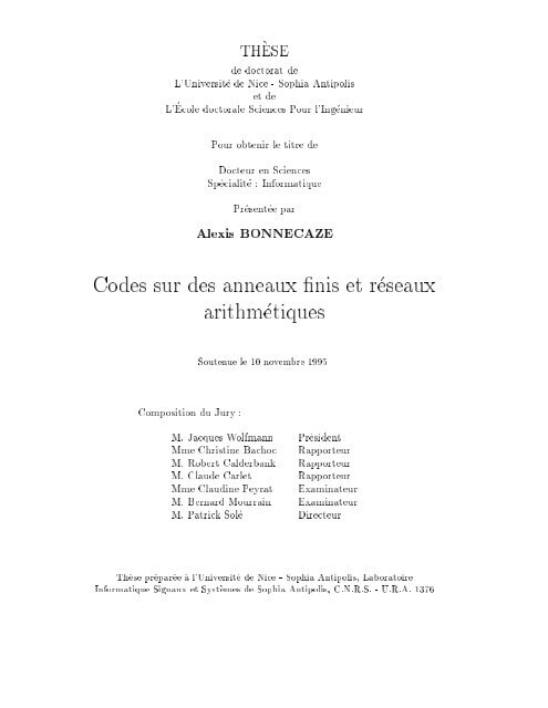
l'on note S(t k v). C'est le cas du plan de Fano qui est un 2 ; (7 3 1) design. Plus
generalement, le plan projectif d'ordre n estun2; (n 2 + n +1n+1 1) design.
3
1
0
2
Figure 1.1: Le plan projectif d'ordre 2
Theoreme 1.5 Considerons un t ; (vk ) design. Alors pour tout entier s tel que
0 s t, le nombre s de blocs contenant s points distincts est independant des s
points:
s =
6
(v ; s)(v ; s ; 1) :::(v ; t +1)
(k ; s)(k ; s ; 1) :::(k ; t +1) :
Par de nition t = .Lesentiers s peuvent ^etre determines a partir de la recurrence
s =
(v ; s)
(k ; s) s+1:
Corollaire 1.3 Dans un t ; (vk ) design, le nombre total de blocs est
b =
!
v
t
!
k
t
4
5

26 CHAPITRE 1. PRELIMINAIRES MATHEMATIQUES
et chaque point appartient a exactement r blocs, ou
et lorsque t =2,ona
bk = vr
r(k ; 1) = (v ; 1):
Bien sur le fait que s soit toujours un entier implique certaines contraintes sur les
parametres.
De nition 1.5 Considerons un t ; (vk ) design. Soient P 1::: Pk les points appartenant
a un des blocs. Considerons les blocs qui contiennent P 1::: Pj mais pas
Pj+1::: Pi pour 0 j i: Alors, si le nombre deces blocs est constant et independant
du choix de P 1::: Pi, on le note ij .
L'entier ij etant independant duchoix des Pi, il est donc egal au nombre de blocs qui
contiennent P 1::: Pj mais pas Pj+2::: Pi+1: Ces blocs peuvent ^etre scindes en deux
familles, suivant qu'ils contiennent ounonPj+1. Ainsi,
ij = i+1j + i+1j+1
et pour tout t ; (vk ) design on peut former le \triangle de Pascal" de ces ij:
1.2.2 Le code de Golay binaire
00 = o
10 = 0 ; 1 11 = 1
20 = 0 ; 2 1 + 2 21 = 1 ; 2 22 = 2
:::
Le code de Golay binaire joue, pour de multiples raisons, un r^ole apartdanslatheorie des
codes. Nous allons etudier plus en detail ces proprietes pour pouvoir mieux comprendre
par la suite son relevement de Hensel sur Z 4. Rappelons que les parametres [n,k,d] d'un
code representent respectivement la longueur, la dimension et la distance minimale du
code.
De nition 1.6 Le code de Golay G 23 est le code residu quadratique de longueur 23. Il
acomme polyn^ome generateur h(X) =X 11 + X 9 + X 7 + X 6 + X 2 + X +1
Le code G 23 est donc lineaire et cyclique. On obtient le code de Golay etendu G 24 en
ajoutant unsymbole de parite a la matrice de G 23 de telle sorte que le code soit autodual
(G 24 = G ? 24). Par construction, le mot 1 appartient a G 24. La distribution de poids
de G 24 est
i : 0 8 12 16 24
Ai : 1 759 2576 759 1
Nous utilisons la notation de Sloane dans [MS77] et[CS88].

1.2. LE CODE DE GOLAY BINAIRE 27
et celle de G 23 est
i : 0 7 8 11 12 15 16 23
Ai : 1 253 506 1288 1288 506 253 1
Le code G23 a pour parametres [23,12,7], il permet donc de corriger trois erreurs. Puisque
la distance minimum est 7, les cosets de poids minimum 3sontdisjoints. Le nombre
de tels cosets est
1+
23
1
!
+
23
2
!
+
23
3
!
=2 11 =2 23;12
et ils representent ainsi tous les cosets de G 23. LecodedeGolay G 23 est donc un code
parfait.
De nition 1.7 Un mot de poids 8 de G 24 est appele une octade.
Theoreme 1.6 Tout vecteur binaire depoids 5 et de longueur 24 est couvert par exactement
un mot de G 24 de poids 8.
Preuve. Si un vecteur de poids 5 etait couvert par 2 octades, alors la distance ! du code
8
serait inferieure ou egale a6. En fait, chaque mot de poids 8 couvre vecteurs
5
distincts de poids 5 et nous avons
759
8
5
!
=
Corollaire 1.4 Les mots de poids 8 (les octades) de G 24 forment un systeme de Steiner
S(5 8 24). Les autres systemes de Steiner contenus dans le code sont S(4 7 23),
S(3 6 22) et S(2 5 21):
Preuve. L'existence du systeme de Steiner se deduit du theoreme precedent. Witt
a montre que deux systemes S ; (5 8 24) di erent seulement parunreetiquetage de
points. Ainsi, S ; (5 8 24) est unique. 2
Theoreme 1.7 Les ij pour le systeme de Steiner forme par les octades sont
i # 0 759
1 506 253
2 330 176 77
3 210 120 56 21
4 130 80 40 16 5
5 78 52 28 12 4 1
6 46 32 20 8 4 0 1
7 30 16 16 4 4 0 0 1
8 30 0 16 0 4 0 0 0 1
24
5
!
:
2

28 CHAPITRE 1. PRELIMINAIRES MATHEMATIQUES
Remarque. Les mots de poids 16 dans G 24 forment un5; (24 16 78) design. La
presence du mot 1 dans le code donnant une certaine symetrie.
Les mots de poids 12 ou dodecades forment aussi un 5-design (5 ; (24 12 48), voir
[MS77], chap 2).
Comme tout code residu quadratique, le code de Golay G 24 est laisse invariant parle
groupe lineaire special PSL 2(q) avec ici q = 23 (C'est un sous groupe distingue du
groupe lineaire des automorphismes de determinant 1).
Soit = f0 1::: 22 1g l'ensemble des etiquettes representant les coordonnees
du code. La derniere coordonnee contenant lesymbole de parite. Soit Q l'ensemble
constitue de 0 et des residus quadratiques et N son complementaire sur la ligne projective.
Q = f0 1 2 3 4 6 8 9 12 13 16 18g
N = f1 5 7 10 11 14 15 17 19 20 21 22g:
Le cardinal de ces deux ensembles est 12. Le code de Golay peut se de nir de maniere
plus \ensembliste". Considerons la permutation de :
: x ! x +1 (mod 23):
En appliquant , l'ensemble N produit 23 12-uplets N 1N 2:::N 12 ou Ni contient les
nombres de la forme n + i (n 2 N): A partir de ces ensembles et en prenant leur
di erence symetrique, on obtient 2 12 ensembles que l'on appelle des C-ensembles (Csets
en anglais). Si on remplace chaque ensemble par sa fonction caracteristique, alors
les C-ensembles correspondent aux mots du Golay etendu.
Puisque N 1 + N 2 + :::N 12 = (la notation + signi ant ici la di erence symetrique),
est lui-m^emeunC-ensemble, et les C-ensembles arrivent en paires complementaires. En
fait, les C-ensembles comprennent l'ensemble vide et son complementaire 759 octades
et leurs complementaires (les 16-uplets), ainsi que 2576 dodecades.
Le groupe PSL 2(23) a pour ordre 6072 et est engendre par les trois permutations suivantes
de :
S : i ! i +1
V : i ! 2i
T : i !; 1
i :
En d'autres termes,
S = (1)(0 1 2 ::: 22)
V = (1)(0)(1 2 4 8 16 9 18 13 3 6 12)
(5 10 20 17 11 22 21 19 15 7 14)
T = (1 0)(1 22)(2 11)(3 15)(4 17)(5 9)(6 19)
(7 13)(8 20)(10 16)(12 21)(14 18):
De nition 1.8 Le groupe de Mathieu M24 est le groupe engendre par S V T et W ,
ou W est de ni de la maniere suivante
W :
8
><
>:
1!0 0 !1
i !;( 1
2 i)2 si i 2 Q
i ! (2i) 2 si i 2 N

1.2. LE CODE DE GOLAY BINAIRE 29
Remarque. W peut aussi s'ecrire
W = (1 0)(3 15)(1 17 6 14 2 22 4 19 18 11)
(5 8 7 12 10 9 20 13 21 16):
Theoreme 1.8 M 24 est le groupe de toutes les permutations de qui laissent xes les
octades du code de Golay G 24:
Le groupe de Mathieu est 5-transitif et transitif sur les octades de G 24. Son cardinal est
759:322560 = 244823040 .
Remarque. Le code de Golay [23, 11] peut aussi ^etre decrit a l'aide de la fonction
trace.
Soit une racine 23 ieme de 1 sur F 2. L'ordre multiplicatif de 2 modulo 23 est 11. Il
existe donc une racine primitive de F 2 11 telle que = 89 (car 2 11 ; 1=89:23). On
peut ecrire
x 23 ; 1=(x ; 1)m (x)m 5(x)
ou m et m 5 designent respectivement le polyn^ome minimal de et 5 .
Le code de Golay [23, 11] a pour polyn^ome generateur . Ses mots peuvents'ecrire
x 23 ;1
(x;1)m
c(a) =(tr(a i )) pour i 2f0:::22g et a 2 F 2 11
et ou trrepresente la fonction trace de F 2 11 sur F 2.
Le groupe de Mathieu M 23 est alors l'ensemble des automorphismes vectoriels de F 2 11
qui conservent l'ensemble des racines 23 iemes de l'unite.
1.2.3 Le MOG
La meilleure facon de travailler avec les mots de G 24 est de les mettre sous la forme
d'un tableau 6 4, appele Miracle Octad Generator, ou MOG. L'inventeur du MOG,
R. T. Curtis [Cur73] et [Cur76], avait besoin d'un outil pratique pour ses recherches sur
le groupe de Mathieu. L'introduction de l'hexacode par Norton [Nor80] puis Conway
[Con81] facilita grandement les calculs sur le groupe de Mathieu. Le MOG permet de
visualiser les mots du Golay. Il permet en outre de
trouver toutes les octades du Golay,
retrouver une octade a partir de 5 points donnes,
veri er si un mot appartient auGolay,
decoder le Golay.
Nous decrivons dans un premier temps la construction de l'hexacode et du MOG, puis
nous donnons quelques exemples permettant de comprendre l'utilisation du MOG.
Considerons le corps F 4 = f0 1!!g, muni des relations 1 + ! = ! 1+! =
! ! + ! = !! =1 ! 2 = ! ! 2 = ! ! 3 =1:

30 CHAPITRE 1. PRELIMINAIRES MATHEMATIQUES
De nition 1.9 L'hexacode C 6 est un code sur F 4 de parametres [6, 3, 4] et de matrice
generatrice 2
6
4
0 0 1 1 1 1
0 1 0 1 ! !
1 0 0 1 ! !
L'hexacode contient donc 64 mots. A n de mieux cerner les symetries, on a pris l'habitude
de representer les 6 symboles d'un mots en trois paires. Les 64 mots peuvent ^etre
obtenus a partir des 5 mots
3
7
5 :
0 1 0 1 ! !
! ! ! ! ! !
0 0 1 1 1 1
1 1 ! ! ! !
0 0 0 0 0 0
en permutant les trois paires, en inversant tout nombrepairdepairesetenmultipliant
par n'importe qu'elle puissance de !. Ces symetries engendrent un groupe d'ordre 72.
Les 5 mots ont respectivement 36, 12, 9, 6, 1 images. Connaissant ces5representations,
on peut deduire que le poids minimum de l'hexacode est 4. Un mot du code est parfaitement
determine par la donnee de trois coordonnees. Le meilleur moyen de determiner
un mot a partir d'une information partielle est de proposer une solution et de la justi er.
Un elementdeF 4 peut ^etre represente par un vecteur binaire de longueur 4. Un mot
de l'hexacode peut donc ^etre represente par un tableau 6 4. Dans un tableau, une ligne
ou colonne est dite paire (resp impaire) si le nombredenon-zeros dans la ligne ou la
colonne est pair (resp impair). La gure 1.2 montre les di erentes interpretations paires
et impaires. Par exemple, le symbole 0 peut s'ecrire 0 ou 1 + ! + ! en representation
impaire et 0 + 1 + ! + ! en representation paire.
Un mot de G 24 peut ^etre obtenu a partir des mots de C 6 de deux manieres di erentes
En remplacant chaque symbole par une interpretation impaire et de maniere que
la premiere ligne deviennent impaire.
En remplacant chaque symbole par une interpretation paire et de maniere que la
premiere ligne deviennent paire.
Ainsi, a partir d'un mot de l'hexacode, on peut construire plusieurs mots du Golay.
Il existe une methode simple permettant deveri er qu'un mot appartient ou non au
Golay. Elle consiste a calculer le compteur pour chaque colonne et pour la premiere
ligne, et le score pour chaque colonne. Dans l'exemple suivant,
0 2 0 2 2 2
0 4
1
!
!
0 1 0 1 ! !

1.2. LE CODE DE GOLAY BINAIRE 31
0
1
!
!
0
1
!
!
0 1 ! ! 0 1 ! !
(a) (b)
Figure 1.2: (a) Interpretation impaire. (b) Interpretation paire.
les compteurs, qui comptent lenombre de non-zeros dans les colonnes, sont respectivement
0 2 0 2 2 2 et le compteur qui compte le nombre de non-zeros dans dans la
premiere ligne est 4. Les scores sont respectivement 0 1 0 1!!. Si les compteurs ont
tous la m^eme parite et que les scores forment unmotdeC 6, (ce qui est le cas ici) le
MOG represente un C-ensemble (c'est a dire l'ensemble des places ou un mot du Golay
a ses elements non nuls).
Exemple A:
Le mot suivant correspond a un mot du Golay
car les compteurs sont tous impairs et les scores 1 0 !!01representent un mot de
l'hexacode:
1 1 1 3 1 1
3
1 0 ! ! 0 1
Exemple B:
Comment completer ce mot de maniere a ce qu'il corresponde a une octade du Golay?

32 CHAPITRE 1. PRELIMINAIRES MATHEMATIQUES
A partir de 5 points donnes, il n'existe qu'une seule possibilite pour construire une octade
car celles-ci forment unsysteme de Steiner S(5 8 24). Si l'on essaye une representation
impaire, on s'apercoit qu'aucune solution ne convient. Avec une representation paire,
on obtient:
2 0 2 0 2 2
2
! 0 ! 0 ! 1
Remarque. Il est a noter que Pless a decode lecodedeGolay en utilisant l'hexacode
et le MOG (voir [Ple86]). Le MOG est donc un outil tres pratique pour travailler dans
M 24. Il permet une visualisation des permutations du groupe ce qui est tres appreciable
compte tenu de la cardinalite deM 24.
Le code de Golay peut ^etre de ni comme etant le code engendre par les images de Q
par les homographies de PSL 2(23). Notons que, modulo 23,
Q = f0 1 2 3 6 4 8 9 12 13 16 18g
= f0 1 2 3 4 ;5 6 ;7 8 9 ;10 ;11g:
Choisissons le C-ensemble correspondant a Q comme le montre la gure suivante. Ecrivons
ensuite les 12 nombres (de 0 a 11) dans l'ordre, avec un signe negatif lorsque le
nombre appartient a N (le complementaire de Q) .
0 1 2
3 4 ;5
6 ;7 8
9 ;10 ;11
Les nombres restants sont places en faisant agir la permutation : z 7! ; 1.
On z
obtient ainsi le MOG standard (standard MOG labeling):
0 1 1 11 2 22
19 3 20 4 10 18
15 6 14 16 17 8
5 9 21 13 7 12
L'idee de base qui sert pour la representation des octades et que chaque octade est une
union de 2 tetrades (les tetrades etant des mots de poids 4).
De nition 1.10 Un sextet est une collection de 6 ensembles de cardinalite 4, tel que
l'union de 2 de ces ensembles forme une octade. Le sextet standard estcelui dont les 6
ensembles sont les colonnes du MOG.
Curtis remarqua que chaque octade rencontrant labriquedegauche en 4 points est
decrite dans l'un des 35 sextets (voir [CS88] gure 11.17, chap. 11). Sa methode permet
de retrouver toutes les octades du Golay.

1.3. THEORIE DES INVARIANTS 33
1.3 Theorie des invariants
Les codes binaires auto-duaux (ou formellement auto-duaux) ont ete abondamment
etudies ([CS90],[War76], [MS73],[Tsa92],[KP92], etc.). Ils admettent souvent de bons
groupes d'automorphismes et ont des proprietes de divisibilite des poids des mots. Particulierement
importants sont les codes de type II, aussi appeles codes pairs auto-duaux
(even self-dual codes, en anglais). Les residus quadratiques de longueur 8m ; 1font
partie de cette famille de codes. A l'image du Golay, ilscontiennent souvent des designs
et ont de gros groupes d'automorphismes.
Parallelement, il est naturel d'etudier les codes de type II quaternaires (sur Z 4). Ils
se de nissent demaniere similaire et se revelent extr^emement interessants. Nous les
etudierons dans le chapitre 5. Nous verrons qu'ils permettent de construire des codes binaires
formellement auto-duaux non lineaires, comme par exemple le code de Nordstrom-
Robinson en longueur 16. Nous rappelons tres brievement les grandes lignes de la theorie
des invariants qui nous sera utile lors de l'etude des codes de type II.
1.3.1 Theorie des invariants
Le theoreme de Gleason (voir [Gle70]) impose des contraintes sur l'enumerateurs de poids
des codes auto-duaux binaires de longueur N. Il donne ainsi une forme generale de ces
enumerateurs de poids qui sont des polyn^omes homogenesdedegre N. La theorie qui
permet d'obtenir ces resultats peut ^etre utilisee dans le cadre de l'etude des codes quaternaires.
C'est la theorie des invariants. Elle fut developpee au dix-neuvieme siecle et
fut surtout utilisee en combinatoire, mais elle a bien d'autres applications en particulier
dans le domaine des mathematiques et de la physique (geometrie, vision, mecanique,:::).
Elle nous est utile ici pour determiner les enumerateurs de poids de certains codes quaternaires
auto-duaux.
C'est Klemm [Kle89] qui le premier a etudie les conditions satisfaites par les enumerateurs
de poids complets de codes auto-duaux sur Z 4. Certaines transformations lineaires
(dont la transformation de MacWilliams) determinent un groupe de substitutions G.
Ce groupe est constitue par des matrices m m a coe cients complexes. Il laisse xe
des polyn^omes homogenes, appeles invariants. En d'autres termes, le groupe G agit sur
l'anneau C[X 1 :::Xm] depolyn^omes. Nous avons:
G C[X 1 :::Xm] ;! C[X 1 :::Xm]
(A f) 7;! A(f)
avec (A(f))(X) =f(A tr X) pour X 2 C N ou tr designe la transposee et la composition.
L'anneau des invariants de G est:
R(G) =ff 2 C[X 1 :::Xm] j A(f) =f 8A 2 Gg
Le nombre d'invariants depend evidemment du cardinal du groupe G: rajouter des
elements dans le groupe fait reduire le nombre d'invariants.

34 CHAPITRE 1. PRELIMINAIRES MATHEMATIQUES
En 1897, Molien a montre que la serie de Hilbert de l'anneau R(G) est
S( )= 1
jGj
X
A2G
1
(1.5)
det(I ; A)
ou jGj designe le nombre de matrices dans le groupe G et det le determinant.
Cette serie, qui a pris le nom de serie de Molien, peut s'ecrire sous la forme
N 0 + N 1
+ N 2
2 + :::+ Ni
i + :::
et permet de conna^tre le nombre Ni de polyn^omes homogenes lineairementindependants
de degre i.
Il est important, pour avoir une meilleure vision de l'anneau des invariants, de pouvoir
en determiner une bonne base (voir [MS77] page 614) de maniere alede nir totalement.
Avant dede nir la notion de bonne base, rappelons que des polyn^omes f 1 :::fm
sont appeles algebriquement dependants s'il existe un polyn^ome P en m variables a
coe cients complexes non tous nuls, tel que
P (f 1:::fm) =0:
Le nombredepolyn^omes algebriquementindependants dans G est donne par le theoreme
suivant:
Theoreme 1.9 Tout groupe ni de matrices G GL(C m ) admet m invariants
algebriquement independants.
Une base de Cohen-Macaulay que l'on notera M(G), est une bonne base car elle donne
une ecriture unique de chaque invariant deG.
De nition 1.11 Une base de Cohen-Macaulay est constituee de l polyn^omes f1 :::fl (l
m) homogenes invariants ou f1 :::fm sont algebriquement independants, tels que
(
C[f1 :::fm] si l = m
M(G) =
C[f1 :::fm] fm+1C[f1 :::fm] ::: flC[f1 :::fm] si l > m
la notation designant la somme directe usuelle.
Tout invariant deG peut ainsi ^etre ecrit comme un polyn^ome en f 1 :::fm si l = m, ou
comme un tel polyn^ome plus fm+1 fois un autre tel polyn^ome etc....
Les polyn^omes f 1 :::fm sont appeles les generateurs primaires et les fm+1 :::fl les
generateurs secondaires. Cette ecriture est appelee decomposition d'Hironaka.
Lorsque l>mil existe des equations polyn^omiales entre les f 1 :::fl du fait de leur
dependance. Ces relations algebriques sont appelees syzygies. Les generateurs secondaires
doivent former un ensemble de cardinalite minimale l qui, avec f 1:::fm engendre
l'anneau en tant que C-algebre. Pour un groupe G donne, il existe plusieurs
decompositions d'Hironaka. Les degres des generateurs primaires et secondaires ne sont
pas uniques. Par contre le nombre t de generateurs secondaires ainsi que leurs degres
e 1:::et peuvent ^etre deduits a partir des generateurs primaires (ou plus exactement
de leur degre). L'entier t est le rang de l'anneau en tant queC[f 1:::fm]-module libre.

1.3. THEORIE DES INVARIANTS 35
Proposition 1.1 Soit d 1d 2:::dm les degres des di erents generateurs primaires d'un
groupe de matrices G. Alors
(a) le nombre degenerateurs secondaires est
t = d1d2 :::dm
jGj
(b) les degres (avec leurs multiplicites) des generateurs secondaires sont les exposants
de la fonction generatrice
S( ):
mY
i=1
(1 ; di )= e1 + e2 + :::+ et :
Il a ete prouve [ZS60] que pour tout groupe ni de matrices m x m a coe cients complexes,
il existe toujours un base de Cohen-Macaulay pourlesinvariants de G. En d'autres
termes les anneaux d'invariants sont Cohen-Macaulay.
Un autre avantage d'avoir une bonne base de l'anneau R(G) est qu'il permet de retrouver
la serie de Molien de G. En e et celle-ci peut toujours s'ecrire sous la forme suivante:
Soit di le degre defi,
S( ) =
8
><
>:
Q 1
m
i=1 (1; d si l = m
i )
Pl d
1+
j
Q j=m+1
m
i=1 (1; di ) sil>m:
(1.6)
Reciproquement, il n'est pas vrai de dire que l'on peut deduire une bonne base de l'anneau
a partir de la serie de Molien puisque Stanley a montre (voir [MS77] page 616) que
l'ecriture (1.6) n'est pas unique.
1.3.2 Le package Invar de Maple et le logiciel Macaulay
Gregor Kemper a developpe lepackage Invar de Maple. Ce package determine l'anneau
des invariants d'un groupe de permutations ou d'un groupe lineaire ni sur Q (ou une
extension de Q).
La fonction invring: Plusieurs fonctions sont disponibles mais la principale fonction
s'appelle invring. Elle est basee sur le theoreme suivant (voir [HR74] pour la preuve).
Theoreme 1.10 Soit K un corps de caracteristique 0 et G un sous groupe ni du groupe
lineaire general de dimension m. Soit K la cloture algebrique de K et R(G) l'anneau
des invariants de G. Nous avons:
(a) Il existe des invariants s 1:::sm 2 R(G), homogenes qui satisfont la propriete
suivante (P):
pour tout 1::: m 2 K,
si( 1::: m) =08i =1:::m , 1 = :::= m =0:

36 CHAPITRE 1. PRELIMINAIRES MATHEMATIQUES
(b) Pour les invariants s 1:::sm 2 R(G), les propositions suivantes sont equivalentes:
(i) Les si satisfont la propriete (P).
(ii) Les si sont algebriquement independants sur K et R(G) est un module libre
de rang ni sur K[s 1:::sm] ayant une base d'invariants homogenes.
(c) Supposons que (ii) de (b) soit satisfait. Nous avons donc R(G) = m0
i=1A fi avec
A = K[s 1:::sm] et fi 2 R(G). Soit i le degre desi et i celui de fi, alors la
serie de Molien S( ) de R(G) est:
S( ) =
1 + :::+ m0
(1 ; i) :::(1 ;
La fonction calcule d'abord la serie de Molien par la formule (1.5). Elle l'ecrit sous la
forme (1.6) et cherche une base de Cohen-Macaulay en utilisant le (c) du theoreme.
Malheureusement, la fonction invring fait appel aux bases de Grobner pour resoudre ses
systemes. Elle utilise de ce fait beaucoup de memoire car les algorithmes que maple
utilise pour les calculs sur les bases standards sont tres lents. Ainsi, il est utopique de
vouloir lui faire calculer une base si le groupe est trop gros (plus de 1000 elements). Le
calcul a la main a ici l'avantage de prendre en consideration les proprietes de chaque
groupe et ainsi de simpli er les methodes de calcul.
Cependant, il existe un logiciel specialise dans les calculs des bases de Grobner:
Macaulay. Ce logiciel est gratuit et peut ^etre rapatrie par ftp. Il admet un grand nombre
de fonctions permettantdedeterminer les invariants d'un anneau assez rapidement. Nos
calculs concernant la caracterisation des enumerateurs de poids des codes de typeIIont
ete veri es a l'aide des logiciels Macaulay et Gap.
m) :

Chapitre 2
Codes quaternaires
L'objet de ce chapitre est d'etudier les codes lineaires sur Z 4 ainsi que leurs releves par
le lemme de Hensel.
2.1 Notions de base
De nition 2.1 Un code en blocs lineaire Cm de longueur N sur Zm est un sous espace
vectoriel de Z N m .
Par la suite, nous allons restreindre notre etude aux codes en blocs lineaires sur Z 4.
De nition 2.2 Un code quaternaire C 4 de longueur N est un code en bloc lineaire sur
Z 4, qui est un sous groupe additif de Z N 4 .
La metrique de Hamming n'est pas su samment precise lorsque l'on travaille sur Z 4,
car elle ne di erencie pas les elements de l'anneau. Dans l'anneau des entiers modulo 4,
l'inverse additif de 1 est 3.
Les elements inversibles 1 et 3 (=-1) jouent unr^ole symetriques dans l'anneau. La
metrique la plus adaptee est la metrique de Lee. SurZ 4, Les di erents poids de Lee sont
i Poids de Lee
0 0
1 1
2 2
3 1
Plus generalement, le poids de Lee peut ^etre de ni sur Zq. le poids de Lee d'un element
x 2 Zq est
WLee(x) = x si x b q
2 c
= ;x sinon
Le poids de Lee d'un vecteur u 2 Z N 4 , wtL(u), est la somme des poids de Lee des
composantes de u. Cette fonction poids permet de de nir la metrique de Lee dL( )sur
37

38 CHAPITRE 2. CODES QUATERNAIRES
Z N 4 : dL(u v) =wtL(u ; v) uet v etant deux vecteurs de Z N 4 .
Cette metrique generalise celle de Hamming dans le cas binaire.
Le produit scalaire surZ N 4 est de ni par (a b) =a 1b 1 + + aNbN (mod 4). Il nous
permet de de nir la notion de dualite entre deux codes quaternaires:
C ? 4 = fu j (u v) 0(mod 4) 8v 2 C 4g:
Le code est dit autodual s'il est egal a son dual (C4 = C ? 4 )etfaiblement autodual s'il est
inclus dans son dual (C4 C ? 4 ).
Exemple: Le code C de matrice generatrice
est autodual de longueur 4.
2
6
4
3 1 1 3
2 2 0 0
0 2 2 0
Notons que Conway et Sloane donnent dans [CS93] une classi cation des codes quaternaires
faiblement auto-duaux engendres par des tetrades (mots de la forme 1 4 0 N;4 ).
Ils montrent que ces codes quaternaires sont equivalents a une somme directe de certains
codes de base. La notion d'equivalence est ici sensiblement plus large que dans le cas
des codes binaires. Dans le cas binaire, deux codes sont equivalents si leurs matrices
generatrices se deduisent l'une de l'autre par des permutations. La structure de l'anneau
Z 4 nous fait considerer non plus les permutations de colonnes dans la matrice generatrice
mais les permutations signees (permutations et eventuellementchangement de signe des
colonnes).
De nition 2.3 Deux codes sont equivalents s'ils possedent deux matrices generatrices
se deduisant l'une de l'autre par des permutations signees. Lorsque les deux matrices
di erent l'une de l'autre par une seule permutation, les codes sont appeles permutationequivalents.
Les codes quaternaires sont desZ4-modules. CesZ4-modules n'etant pas forcement
libres, ils n'admettent pas toujours une base. Cependant ([HKC + 94]), tout code quaternaire
est permutation-equivalent auncodeC4 dont la matrice generatrice est de la
forme:
G = Ik1 M N
(2.1)
0 2Ik2 2P
Ou M et P sont des matrices binaires et N une matrice a coe cients sur Z 4. Le code
contient donc4 k1 2 k2 mots et sa dimension dim(C4) surZ 4 est donnee par:
dim(C 4) = log 4 jC 4j = log 4(4 k1 2 k2 )=k1 + k 2=2 :
Le code C4 est libre si et seulement sik2 =0. SiC4 a pour matrice generatrice G, le
code dual C ? 4 a pour matrice generatrice:
3
7
5
G = ;N tr ; P tr M tr P tr IN;k1;k2
2M tr 2Ik2 0

2.1. NOTIONS DE BASE 39
et contient4 N;k1;k2 2 k2 mots de code. Dans l'exempleprecedent, C est un code auto-dual
de dimension 2, il contient donc 16 mots et est de longueur 4.
Un code est dit isodual s'il est equivalent a son dual.
L'automorphisme de groupe Aut(C 4)deC 4 consiste en toutes les permutations signees
sur les coordonnees qui preservent l'ensemble des mots du codes.
2.1.1 Enumerateurs de poids
Il existe plusieurs emumerateurs de poids (et distances) associes a C 4. Dans [Cam79], P.
Camion introduit la notion d'enumerateur de poids exact qui de nit totalement le code.
L'enumerateur de poids exact d'un code quaternaire est un polyn^ome en les variables
Xjk (j =0 1 2 3 k =1:::N):
eweC4(Xjk) = X
NY
a2C4 k=1
et l'enumerateur de distances exact est de ni par:
edeC4(Xjk) = 1
jC 4j
X
NY
ab2C4 k=1
Xa kk
Xa k;b kk:
Notons que le code C 4 est lineaire si et seulement silesemumerateurs de poids et de
distances exacts sont identiques. En e et, C 4 est lineaire si et seulement si pour chaque
mot c 2 C 4, il existe une paire ordonnee (b c) telle que a = b ; c.
Remarque. La di erence entre les notions de linearite et de distance invariante peut
^etre decrite de la facon suivante:
Cestlineaire , ewe(a + C) =ewe(C) a 2 C
C est de distance invariante , we(a + C) =we(C) a 2 C
ou we represente la distribution de poids de Hamming.
Lorsque seule la composition des mots nous interesse (et non la place des elements dans
le mot), on identi e les variables Xjk (k =1:::N)avec Xj. On obtient un polyn^ome
en quatre variables X0 X1 X2 X3. Lorsque nous n'utilisons pas l'enumerateur de
poids exact, nous adoptons par commodite les notations de [HKC + 94] et [BSC95] et
appelons ces variables respectivement W XYZ.
L'enumerateur de poids complet (ou c.w.e.) de C4 est:
cweC4(WXYZ)= X
a2C4
W n0(a) X n1(a) Y n2(a) Z n3(a) (2.2)
ou ni(a) represente le nombre de composantes de a qui sont congrus a i modulo 4.
Cependant, l'existence de permutations signees nous fera le plus souvent utiliser ici
l'enumerateur de poids symetrique (ou s.w.e), obtenu en identi ant X et Z dans (2.2):
sweC4(WXY)=cweC4(WXYX) :

40 CHAPITRE 2. CODES QUATERNAIRES
Ainsi, deux codes equivalents ont m^eme enumerateur de poids symetrique.
L'enumerateur de poids de Lee de C 4 est le polynome homogene de degre 2N:
LeeC4(WX) = P u2C4 W 2N;wt L(u) X wt L(u)
= sweC4(W 2 WXX 2 ) :
L'enumerateur de poids de Hamming de C 4 est de ni par:
HamC4(WX)=sweC4(WXX) :
Soit C4 un code quaternaire. Notons C0 4 le code raccourci obtenu enenlevant une
coordonnee a C4 et C00 4 le sous code de C0 4 de poids de Lee pair. De plus, notons
A(n0n1n2) le nombre de mots de la forme W n0 n1 n2 X Y .
Theoreme 2.1 Supposons que le groupe d'automorphisme de C 4 agisse transitivement
sur les N positions des coordonnees. Si le poids de Lee minimum dans C 4 est au moins
trois alors
et
sweC0 1
(WXY) =
4 N
sweC00 1
(WXY) =
4 N
@
@W
@
@X
+ @
@X
+ @
@Y
!
!
@
+
@Y
sweC4(WXY)
sweC4(WXY) :
Preuve. Considerons le tableau constituedesA(n 0n 1n 2) mots de la forme W n0 X n1 Y n2
dans C 4. Cet ensemble de mots represente l'orbite d'un mot de cette forme par l'action
du groupe de permutations. Dans chaque colonne le nombre d'elements egaux a0,1
et 2 est constant et respectivement egal a A(n0n1n2)nk ,pourk 2f0 1 2g. enlever une
N
coordonnee dans le code revient aeliminer une colonne dans le tableau. Le resultat s'en
deduit. 2
De plus si l'automorphisme de groupe de C 4 agit t-transitivementsurlesN positions
de coordonnees, alors pour k =0 1 2,
N(N ; 1) (N ; t +1)j A (n0n1n2)nk(nk ; 1) (nk ; t +1):
2.1.2 Identite de MacWilliams
L'identite de MacWilliams lie l'enumerateur de poids d'un code a celui de son dual.
l'enumerateur de poids d'un code C binaire est le polyn^ome
WC(WX)= X
W N;WH (a) WH (a)
X
a2C
ou WH(a) designe le poids de Hamming de a.
On a
WC(W + X W ; X) = X
b2F N 2
X
a2C
(;1) (ab) W N;W (b) X W (b) :

2.1. NOTIONS DE BASE 41
Si C est lineaire, alors
et on retrouve l'identite de MacWilliams:
et la transformation de MacWilliams
P a2C(;1) (ab) = jCj si b 2 C ?
= 0 sinon
1
jCj WC(W + X W ; X) =W C ?(WX)
P (WX) ! P (W + X W ; X):
Cependant, la transformee de MacWilliams ne caracterise pas les codes lineaires. Il
existe en e et des codes non lineaires dont les enumerateurs de poids satisfont cette
transformee. Les codes de Kerdock et Preparata (voir [MS77], chap 15) en sont lemeilleur
exemple.
L'identite de MacWilliams peut ^etre etendue naturellement au cas quaternaire. Soit
C 4 un code quaternaire, l'enumerateur de poids complet du code dual C ? 4 en fonction
du cweC4(WXYZ) est:
cwe C ? 4 (WXYZ)= 1
jC 4j cwe C4(W +X+Y +Z W+iX;Y ;iZ W ;X+Y ;Z W ;iX;Y +iZ) :
Lorsque le code est auto-dual, l'identite de MacWilliams peut ^etre representee par la
matrice.
2
1
6
1=2
6 1
6
4 1
1
i
;1
1
;1
1
3
1
;i 7
;1 5
1 ;i ;1 i
:
L'enumerateur de poids symetrique du code dual C ? 4 en fonction du sweC4(WXY) est
swe C ? 4
(WXY)= 1
jC 4j sweC4(W +2X + YW ; YW ; 2X + Y ) :
Les equations correspondantes concernant les enumerateurs de poids de Lee et de Hamming
sont
LeeC ? (WX)=
4
1
jC4j LeeC4(W + X W ; X)
Ham C ? 4
(WX)= 1
jC 4j HamC4(W +3X W ; X):
Deux codes sont ditsformellement duaux (ou pseudo duaux) si leurs enumerateurs de
poids veri ent l'identite de MacWilliams. Ces codes ne sont donc pas toujours lineaires.
Cependant Claude Carlet a montre dans [Car] que si l'on considere un code C q-aire,
l'enumerateur de poids exact de C satisfait l'identite de MacWilliams si et seulement
si C est lineaire. Il prouve que (pour j =0:::q; 1 k =1:::N et ! = e 2i =q ), les
propositions suivantes sont equivalentes:

42 CHAPITRE 2. CODES QUATERNAIRES
1. C est lineaire
2. 1
jCj WC( P q;1
s=0 ! js Xsk) a ses coe cients entiers positifs.
3. 1
jCj WC( P q;1
s=0 ! js Xsk) =W C ?:
La notion d'enumerateurs de poids exact est donc plus forte que celle d'enumerateurs de
poids complet. Nous verrons par la suite l'importance de ces notions dans la comprehension
de la Z 4-dualite.
2.2 L'application Gray-map
L'importance grandissante des codes quaternaires est sans nul doute liee a l'application
\Gray-map", qui, a l'origine servait a encoder des sequences avec le systeme QPSK
(Quadrature Phase-Shift Keying).
2
(-1)
1
(i)
(-i)
3
(1)
0
Gray-map
Figure 2.1: Gray-map et encodage de Gray.
De nisons les trois applications de Z 4 sur Z 2 par
c (c) (c) (c)
0 0 0 0
1 1 0 1
2 0 1 1
3 1 1 0
Ces applications peuvent s'etendre a des vecteurs de longueur N, deZN 4 vers Z2N 2 .
L'application Gray-map : ZN 4 ! Z2N 2 est donnee par
(c) =( (c) (c)) c 2 Z N 4 :
Remarque. Le code binaire forme des mots ( (c) (c) (c)) pour c =0 1 2 3, est
lineaire et tous ses poids sont pairs.
11
01
10
00

2.2. L'APPLICATION GRAY-MAP 43
La Gray-map est aussi l'application de Z N 4 vers ZN 2 Z N 2
telle que
(a 1:::aN) 7! ((u 1:::uN) (v 1:::vN))
ou pour tout i 2f1:::Ng ai =2ui +(ui + vi mod 2):
L'image d'un code quaternaire C 4 de longueur N est le code binaire C de longueur 2N.
Le code C est appele l'image binaire de C 4. Il n'est pas forcement lineaire. Cependant,
lorsque C est lineaire et la matrice generatrice de C 4 est de la forme 2.1, alors la matrice
generatrice de C est de la forme (voir [HKC + 94])
2
6
4
Ik1 M (N) Ik1 M (N)
0 Ik2 P 0 Ik2 P
0 0 (N) Ik1 M (N)
L'application Gray-map permet donc de construire des codes binaires a partir de codes
quaternaires. Sa propriete essentielle est d'^etre une isometrie. Ainsi, nous allons voir
que si la disposition des mots dans l'image binaire C ne lui permet pas en general d'^etre
lineaire, C est tout de m^eme de distance invariante.
2.2.1 Proprietes de l'application Gray-map
Theoreme 2.2 L'application Gray-map est une isometrie
3
7
5 :
(Z N 4 Lee distance) ! (Z 2N
2 Hamming distance):
Preuve. A partir de la de nition de la metrique de Lee on a
WH( (c)) = WLee(c) c 2 Z N 4
dH( (c 1) (c 2)) = dLee(c 1c 2) c 1c 2 2 Z N
4
ou WH et dH representent respectivement le poids et la distance de Hamming pour les
mots binaires. 2
L'application ne conserve pas la propriete delinearite. Cependant elle conserve la
propriete de distance invariante car c'est une isometrie:
Theoreme 2.3 Soit C 4 un code sur Z 4 ayant la propriete de distance invariante (avec
la distance deLee). Alors son image binaire (C 4)=C est de distance invariante (avec
la distance de Hamming).
Ainsi, l'image binaire d'un code quaternaire est de distance invariante. Un code C 2 Z 2 2N
est dit Z 4-lineaire s'il peut ^etre de ni comme etant l'image par la Gray-map d'un code
quaternaire, c'est a dire si
N 9 C4 2 Z4 tq (C4) =C:
On a alors la propriete sur les distributions de poids
HamC(WX)=LeeC4(WX)=sweC4(W 2 WXX 2 ):

44 CHAPITRE 2. CODES QUATERNAIRES
Puisque l'image binaire d'un code quaternaire (C 4)=C n'est pas toujours lineaire,
elle n'admet pas de dual au sens algebrique du terme. On de nit alors le Z 4-dual de C
qui est C? = (C ? 4 ): Ainsi, nous avons le diagramme suivant
C 4 ;! C = (C 4)
dual #
C ? 4 ;! C? = (C ? 4 ):
Il n'est pas possible de rajouter une eche notee \dual" dans la partie droite du diagramme
car les 2 codes binaires ne sont que Z 4-duaux. Cependant, la propriete de
Z 4-dualite est plus forte qu'on pourrait le penser a premiere vue:
Theoreme 2.4 Soit C4 un code quaternaire etC ? 4 son dual. Les distributions de poids
de leurs images binaires C = (C4) et C? = (C ? 4 ) satisfont la transformation de
MacWilliams.
Preuve. On a
HamC? (WX) = LeeC ? (WX)
4
= 1
jC4j LeeC4(W + X W ; X)
= 1
jC4j HamC(W + X W ; X):
2.2.2 Conditions de linearite et d'auto-dualite
Nous donnons ici les conditions pour que
1. un code binaire soit Z 4-lineaire,
2. l'image binaire C d'un code quaternaire C 4 soit lineaire,
3. l'image binaire C d'un code quaternaire auto-dual C 4 soit auto-dual.
Pour que C soit Z 4-lineaire, Il faut qu'il existe un code quaternaire C 4 tel que (C 4)=C.
Un mot de C s'ecrit donc (a) =( (a) (a)) a 2 C 4. Mais si (a) est un mot de C,
(;a) l'est aussi. (;a) =( (a) (a)). Ainsi, si C est Z 4-lineaire, il est laisse xe par
l'application
: (a 1a 2:::aNaN +1:::a 2N) 7! (aN +1:::a 2Na 1a 2:::aN) (2.3)
qui permute les parties gauche et droite de a. En d'autres termes peut ^etre representee
par la permutation
(1N + 1)(2N +2):::(N2N):
Notons S le groupe engendre par les transpositions (1N +1) (2N +2):::(N2N):
2

2.2. L'APPLICATION GRAY-MAP 45
Theoreme 2.5 Un code binaire quelconque C de longueur 2N (N 2 N) estZ 4-lineaire
si et seulement si ses coordonnees satisfont
u v 2 C ) u + v +(u + (u)) (v + (v)) 2 C (2.4)
ou est l'application representee en (2.3), et est le produit composantes par composantes
de deux vecteurs.
Preuve. Voir [HKC + 94]. 2
Exemple: Hammons et al. montrent dans[HKC + 94] que le code de Golay binaire G 24
n'est pas Z 4-lineaire. Ils procedent par contradiction en considerant 2 mots u et v de
G 24 qui veri ent
(u + (u)) (v + (v)) =2 g 24 :
Soient
u =
1 1 1 1 0 0
1 1 1 1 0 0
0 0 0 0 0 0
0 0 0 0 0 0
v =
et la permutation representee a la gure 2.2. Alors on a
0 1 1 1 1 1
1 0 0 0 0 0
1 0 0 0 0 0
1 0 0 0 0 0
Figure 2.2: Description de la permutation a l'aide du MOG.
u + (u) =
0 0 1 1 0 0
0 0 1 1 0 0
0 0 1 1 0 0
0 0 1 1 0 0
v + (v) =
1 1 1 1 1 1
1 1 0 0 0 0
0 0 1 1 0 0
0 0 0 0 1 1
et (u + (u)) (v + (v)) est de poids 4 .
Par contre, le code de Nordstrom-Robinson (16 256 6) (voir [FST93]) est lui Z 4lineaire
et peut donc ^etre de ni par une matrice generatrice a coe cients sur Z 4:
Theoreme 2.6 L'image binaire (C 4) d'un code quaternaire C 4 est lineaire si et seulement
si
a b 2 C 4 ) 2 (a) (b) 2 C 4:
:

46 CHAPITRE 2. CODES QUATERNAIRES
Preuve. Le resultat decoule de l'identite
(a)+ (b)+ (a + b) = (2 (a) (b)):
2
Lorsque son image binaire est lineaire, la forme de la matrice generatrice de C 4 est
particuliere. Considerons 2 elements quelconques de coordonnees i 1 et i 2,ayant m^eme
parite entre elles, sur la premiere ligne de la matrice. Alors les elements de coordonnees
i 1 et i 2 ont m^eme parite entre elles sur toutes les lignes.
Exemple: Considerons le code quaternaire C 4 de longueur N = 6 et dimension k =3
engendre par la matrice generatrice
2
6
4
1 2 0 1 3 1
2 1 3 0 1 1
0 1 1 2 2 0
L'image binaire de C 4 est le code C lineaire de longueur N = 12 et dimension k =6
engendre par la matrice
2
6
4
3
7
5
0 1 1 1 0 0 0 1 1 0 0 1
1 0 1 1 0 0 1 0 0 1 1 0
1 1 0 1 1 0 0 0 0 1 0 1
1 1 1 0 0 1 0 0 1 0 1 0
0 0 0 1 0 1 1 1 1 1 0 0
0 0 1 0 1 0 1 1 1 1 0 0
Notons que (toujours dans l'hypothese ou l'image binaire est lineaire) si les ci i 2
f1 kg forment les lignes d'une matrice generatrice d'un code C 4 quaternaire, alors
(ci) (;ci) forment les lignes d'une matrice generatrice de l'image binaire .
L'image binaire (C 4) d'un code quaternaire auto-dual C 4 est auto-duale si et seulement
si la matrice generatrice de C 4 est d'une certaine forme: Considerons 4 elements
quelconques de coordonnees i 1, i 2, i 3 et i 4 de m^eme parite, sur la premiere ligne de la
matrice. Alors les elements de coordonnees i 1, i 2, i 3 et i 4 ont m^eme parite sur toutes les
lignes.
Les mots de C 4 doivent ^etre de longueur multiple de 4 car si l'on considere un mot
c 2 C 4,ona
(c:c) =n 1(c)+n;1(c)(mod 4):
Exemple A: Il existe deux versions du code D 4 de ni dans [CS93]. Leurs matrices
generatrices sont 2
6
4
1 1 1 1
0 2 0 2
0 0 2 2
3
7
5 et
2
6
4
1 3 3 3
0 2 0 2
0 0 2 2
Notons que l'on passe d'une representation a l'autre par des permutations signees. Ces
deux matrices donnent donc deux codes equivalents. Leurs images binaire donnent deux
codes equivalents binaires lineaires et auto-duaux de longueur 8 et dimension 4.
3
7
5 :
3
7
5

2.3. DUALITE FORMELLE ET Z 4-DUALITE 47
Exemple B: Le code 0 8 construit par Conway et Sloane [CS93] a pour matrice generatrice
G 0 8
=
2
6
4
1 1 1 1 0 0 0 2
0 0 0 2 1 1 1 1
0 2 0 2 0 0 0 0
0 0 2 2 0 0 0 0
0 0 0 0 0 2 0 2
0 0 0 0 0 0 2 2
et pour distance minimale 4. D'apres la forme de G 0 8 ,onpeutdeduire que ( 0 8)est
lineaire. Il n'existe que trois codes auto-duaux de longueur 16 et distance minimale
4, parmi lesquels le code F 16 de Pless dans [Ple72]. Les deux autres codes ont une
distribution de poids di erente de celle de F 16. Or ( 0 8)etF 16 ont des distributions de
poids identiques. Ainsi
( 0 8) = F 16:
La matrice generatrice de F 16 est
GF16 =
2
6
4
1 1 1 1 0 0 0 0 0 0 0 0 0 0 0 0
0 0 1 1 1 1 0 0 0 0 0 0 0 0 0 0
0 0 0 0 1 1 1 1 0 0 0 0 0 0 0 0
0 0 0 0 0 0 0 0 1 1 1 1 0 0 0 0
0 0 0 0 0 0 0 0 0 0 1 1 1 1 0 0
0 0 0 0 0 0 0 0 0 0 0 0 1 1 1 1
1 0 1 0 1 0 1 0 0 0 0 0 0 0 1 1
1 1 0 0 0 0 0 0 1 0 1 0 1 0 1 0
2.3 Dualite formelle et Z4-dualite
Les enumerateurs de poids de codes Z 4-duaux satisfont l'identite de MacWilliams car ils
sont images de codes duaux quaternaires par la Gray-map. La notion de Z 4-dualite est
donc plus forte que la notion de dualite formelle. On a
Z 4-dualite ) dualite formelle.
Dans [Car], Claude Carlet remarque que la notion d'enumerateur de poids complet ne
permet pas de faire une distinction entre la Z 4-dualite et la dualite formelle (ou m^eme
la dualite algebrique). La notion d'enumerateur de poids exact est quant a elle trop
forte puisque les images binaires de codes quaternaires ne sont pas, en toute generalite,
lineaires. C. Carlet introduit alors la notion de classe d'equivalence d'enumerateurs de
poids exact. Nous la decrivons tres brievement.
Le cwe d'un code C de longueur 2N peut ^etre obtenu a partir de l'enumerateur de
poids exact en identi ant les mon^omes de C ayant m^eme poids complet. Une maniere
d'identi er ces mon^omes est de considerer des classes d'equivalences. Pour cela, on
considere un groupe de permutations sur f1:::2Ng et l'ideal IG de A = R[Xjk j =
0 1 k =1:::2N], engendre par la famille de polyn^omes
(
2NY
k=1
Xa kk ; 2NY
k=1
3
7
5
Xa k (k)) ou a 2 C et 2 G:
3
7
5

48 CHAPITRE 2. CODES QUATERNAIRES
La classe d'equivalence de l'enumerateur de poids exact de C modulo IG est alors notee
WC=G: Lorsque G represente l'ensemble de toutes les permutations sur f1:::2Ng, il
est clair que l'on obtient lecwedeC.
Intuitivement, le choix du groupe permet de doser la precision de l'enumerateur de
poids, entre le complet et l'exact. Le groupe S de ni dans le paragraphe precedent
correspond a la partition sur f1:::2Ng dont les elements sont les paires fi i + Ng
(i 2f1:::Ng). Les polyn^omes WC=S et DC=S, qui representent respectivement la
classe d'enumerateurs de poids et de distances, sont des polyn^omes en les variables
(X 0kX 1k), pour k 2f1:::Ng:
Theoreme 2.7 1
jCjWC=S( P1 s=0 ! jsXsk) a ses coe cients entiers positifs m^eme si C n'est
pas lineaire. La propriete reste vraie avec DC=S.
Theoreme 2.8 Soient C et C? 2codes Z 4-duaux, alors
et
ou k 2f1:::Ng
DC=S = WC=S DC?=S = WC?=S
1
jCj WC=S(X 0k + X 1kX 0k ; X 1k) =WC?=S(X 0kX 1k)
Au groupe S correspond donc l'enumerateur de poids (on identi e ici la classe avec le
polyn^ome) permettant de faire la distinction entre la Z 4-dualite etladualite formelle.
2.4 Constructions de codes quaternaires
La construction (uju+v) est apparue pour la premiere fois avec Plotkin [Plo60], puis fut
redecouverte par Sloane and Whitehead [SW70] dix ans plus tard. Forney la renomma
\squaring construction" dans [For88]. Soit Ci, i =1 2 un code binaire de parametres
(n Midi). Alors
C = f(uju + v) u 2 C 2v2 C 1g
est un code binaire de parametres (2n M 1M 2 min(2d 1d 2)). Le lemme suivant etudie le
lien avec la Gray-map et les codes quaternaires.
Lemme 2.1 Soient C 1 et C 2 2codes binaires lineaires et soit
C 1 +2C 2 = fv +2u j v 2 C 1u2 C 2g :
Alors C 1 +2C 2 est quaternaire si et seulement si a b 2 C 2 pour tout a b 2 C 1,ou
represente la multiplication composantes par composantes. On a de plus
(C 1 +2C 2)=f(uju + v) u 2 C 2v2 C 1g :

2.5. RELEVEMENTS DE HENSEL DE CODES BINAIRES 49
Preuve. La condition est clairement necessaire. Montrons qu'elle est su sante. Soient
a = a 1 +2a 2, b = b 1 +2b 2 2 C 1 +2C 2,ou a 1b 1 2 C 1 et a 2b 2 2 C 2.Leresultat se deduit
de l'identite
a + b = a 1 b 1 +2[a 2 b 2 (a 1 b 1)]
ou represente l'addition binaire. 2
Exemple A: Soit R 8 le code arepetition de longueur 8, et soit P 8 le code dual de 1 de
longueur 8. Le code Z 4-lineaire R 8 +2P 8 est le code auto-dual 8 que Klemm construit
dans [Kle89] Son image binaire ( 8) est le code auto-dual binaire [16 8 4] que Pless
nomme E 16 dans [Ple72].
Exemple B: Le code de Hamming binaire etendu [8 4 4] note H 8 est (R 4 +2P 4), ou
R 4 est le code arepetition de longueur 4, et P 4 le code pair de longueur 4.
2.5 Relevements de Hensel de codes binaires
De nition 2.4 Un code cyclique C de longueur N sur Zq (q =2 a 1 a 1) est un
code lineaire ayant la propriete suivante:
Si (c 0c 1:::cn;1) 2 C alors (c 1c 2:::cn;1c 0) 2 C:
Si l'on represente les mots de codes par des polyn^omes, les codes cycliques sont les
ideaux de l'anneau Zq[x]=(x N ; 1): Il existe 2 facons de considerer la construction de
codes cycliques sur Zq. Elles correspondent aux notions de \top down approach" et
\bottom up approach" qui sont analysees en detail par R. Calderbank et N. Sloane dans
[CS94]. La premiere approche consiste a considerer l'anneau des entiers 2-adiques puis
areduire modulo 2 a pour obtenir un code sur Z 2 a.
Exemple A: Le code de Hamming 2 adique de longueur 7.
A partir de la factorisation de x 7 ;1modulo2et4,onobtient facilement la factorisation
2-adique
ou
x 7 ; 1=(x ; 1)(x 3 + x 2 +( ; 1)x ; 1)(x 3 ; ( ; 1)x 2 ; x ; 1)
=0+2+4+32+128+256+:::
est un nombre 2-adique satisfaisant l'equation
2 ; +2=0:
Le code 2-adique de longueur 7 et de polyn^ome generateur (x 3 + x 2 +( ; 1)x ; 1) est
le relevement 2-adique du code de Hamming binaire [7,4,3].
Le polyn^ome generateur du code sur Z 4 est x 3 +2x 2 + x ; 1. En etendant cecodepar
un symbole de parite on obtient l'Octacode.
Exemple B: Le code de Golay 2-adique de longueur 23 a pour polyn^ome generateur
x 11 + x 10 +( ; 3)x 9 ; 4x 8 ; ( +3)x 7 ; (2 +1)x 6 ; (2 ; 3)x 5
;( ; 4)x 4 +4x 3 +( +2)x 2 +( ; 1)x ; 1

50 CHAPITRE 2. CODES QUATERNAIRES
ou =0+2+8+32+64+128+::: est un nombre 2-adique satisfaisant l'equation
2 ; +6=0:
Ce polyn^ome permet d'obtenir tous les polyn^omes generateurs des codes de Golay sur
Z 2 a.
L'approche \bottom up" consiste a utiliser plusieurs relevements successifs de maniere
a obtenir un code sur Z 2 a. Pour obtenir un code sur Z 8, il faut ainsi relever 2 fois le
polyn^ome generateur binaire. Dans [CS94], Calderbank et Sloane examinent endetail
les structures des codes cycliques releves sur Z 8 Z 16 jusqu'a l'anneau Z 2 1 des entiers
2-adiques.
Nous utilisons ici l'approche \bottom up" pour construire des codes cycliques quaternaires.
En d'autres termes, nous obtenons nos codes quaternaires en relevant des codes
binaires cycliques. Une question interessante est de savoir quelle incidence produit le
relevement sur les proprietes du code binaire.
De nition 2.5 Un code quaternaire C 4 de longueur N est cyclique si et seulement si
C 4 estunideal dans Z 4[x]=(x N ; 1):
Considerons un code cyclique binaire C engendre par le polyn^ome h 2(x) 2 Z 2[x]. Soit
h(x) 2 Z 4[x] lerelevement de Hensel de h 2(x), et soit C 4 =(h(x)) le code quaternaire
cyclique engendre par h(x). Pour un element a 2 C xe, notons Ca l'ensemble detous
les mots b 2 C 4 tels que b a (mod 2). Si b b 0 2 Ca, alors b ; b 0 2 Ca est un mot dont
tous les elements sont egaux a 0 ou 2. Ainsi, b ; b 0 =2c ou levecteur binaire c est un
mot du code binaire cyclique C. Onadonc
C4 = [
[a +2Ca]
a2C
ou Ca est un coset de C qui depend de a. La somme quaternaire des vecteurs binaires
a et b satisfait
a + b = a b +2a b:
La correspondance qui existe entre les mots a dans C et les cosets Ca de C satisfait
l'identite
Ca b = Ca + Cb + a b
ou represente l'addition binaire, et la multiplication composantes par composantes.
Cette correspondance joue un r^ole central dans la comprehension du relevement. Il serait
donc utile de l'analyser en detail. Le probleme qui nous interesse est le suivant: Combien
de 2 apparaissent-ils lors du relevement d'un mot binaire? La reponse a cette question
permettrait de connaitre le poids minimal du code releve. L'action de relever induit-elle
toujours une progression du poids minimal? Sinon, quelle condition faut-il pour que le
releve d'un code binaire C ait un poids de Lee superieur a celui de C?

2.6. IDEMPOTENTS DES CODES CYCLIQUES QUATERNAIRES 51
2.6 Idempotents des codes cycliques quaternaires
Calderbank et Sloane [CS94] ont montre que tout code cyclique quaternaire est de
la forme (f2g) ou 2g divise 2f Lorsque 2g = 2f, le code cyclique est engendre
par un polyn^ome unique f. Dans [PQ95], Vera Pless et Zhongqiang Qian prouvent
independamment que tout code cyclique quaternaire admet des generateurs de l'une des
formes suivantes
(f) (2g) (fh2fg)ou fgh = x N ; 1 sur Z 4:
Ce resultat permet de determiner facilement les generateurs du code dual.
Nous donnons ici un resultat general concernant les idempotents des codes cycliques
quaternaires engendres par un seul polyn^ome f.
Lemme 2.2 Soit g 2 le polyn^ome generateur d'un code cyclique binaire (g 2) et soit g le
relevement de Hensel de g 2.
(1) Considerons f 2 (g) tel que f 2,lareduction modulo 2 de f, engendre lecode
cyclique binaire (g 2).
Alors (f) =(g).
(2) j(g)j = j(g 2)j 2 .
(3) Soit 2 l'idempotent du code cyclique binaire (g 2) et soit 2 Z 4[x] tel que
2 (mod 2). Alors = 2 est l'unique generateur idempotent de g.
Preuve. Pour montrer (2) il su t d'observer que g et g 2 sont des polyn^omes unitaires
de m^eme degre.
Pour prouver (1) on considere l'homomorphisme dereduction modulo 2. Par cette
application, l'image de f est f 2 = g 2, et son noyau inclut (2f) =(2g). Ainsi
et
j(f)j j(2g)j j(g 2)j = j(g 2)j 2
(f) =(g):
Pour prouver (3) on peut ecrire, puisque ( 2)=(g2), que = g +2a pour des
polyn^omes a 2 Z4[x]. Alors = 2 = 2g2 ,et appartient au code cyclique (g).
2
Puisque 2 2 (mod 2), et que 2 engendre (g2), on deduit de (1) que engendre
(g). Puisque 2 (mod 2) on peut ecrire que = 2 = +2b pour un polyn^ome
2 2 b 2 Z4[x]. On a alors = = +2b = et est un idempotent. La preuve de l'unicite
est similaire a celle que l'on peut trouver dans [MS77, Chapitre 8]. 2

52 CHAPITRE 2. CODES QUATERNAIRES

Chapitre 3
Translates des codes quaternaires
Dans ce chapitre, nous nous interessons aux translates des codes quaternaires. Nous
allons voir que la connaissance des enumerateurs de poids des translates de codes est
importante a plus d'un titre. Avec Iwan Duursma, nous proposons une methode pour les
determiner. Pratiquement, et bien qu'elle soit generale, il est di cile de traiter tous les
cas gr^ace a cette methode. Cela est du au fait qu'une partition reguliere de l'ensemble
des syndromes d'un code est souvent di cile a trouver. Nous illustrons notre travail
avec un exemple celebre de famille de codes: Les codes de Preparata.
Nous rappelons dans un premier temps les de nitions des codes de Preparata et Kerdock.
Le chapitre est ensuite entierement consacre a l'article \Translates of linear codes
over Z 4". Il est interessant de constater que les codes triviaux de Preparata (m =1 2,
respectivement) possedent deja les caracteristiques du cas general (pour respectivement
m impair et m pair). Ils admettent tous les deux dix translates d'enumerateurs de poids
complets distincts. De plus, la forme generale des representants des translates se deduit
de celle des cas triviaux.
3.1 Codes de Kerdock, Nordstrom-Robinson, et Preparata
En 1968, F.P. Preparata a construisit une classe de codes binaires optimums pouvant
corriger deux erreurs ([Pre68]). Le code de Preparata, qui n'est pas lineaire, est de
longueur 2 m (m pair), a une distance minimale d = 6 et admet le nombre de mots le
plus important pour ces parametres. Une propriete interessante de ce code est que sa
distribution de poids est la transformee de MacWilliams de la distribution de poids du
code de Kerdock, construit en 1972 (voir [Ker72]). Les codes de Preparata et de Kerdock
sont ainsi formellement duaux. Il existe plusieurs facons de construire ces codes ([MS77],
[Car90], [BvLW83], etc...). La de nition la plus simple du Preparata semble ^etre celle
de Baker ([BvLW83]):
De nition 3.1 Soit un entier m pair 4, m0 = m;1 et un element primitif du corps
de Galois d'ordre 2m0 .Lecode de Preparata P de longueur 2m (m 4) est l'ensemble des
couples (U V ) de parties du corps de Galois d'ordre 2m0,decardinaux pairs et veri ant:
53

54 CHAPITRE 3. TRANSLATES DES CODES QUATERNAIRES
P u2U u = P v2V v
P u2U u 3 + P v2V v 3 =( P u2U u) 3 :
Malheureusement, et de l'aveu m^eme de Van Lint ([vL83]), aucune de ces de nitions ne
permet de comprendre facilement les proprietes de ces codes et jusqu'a 1992, personne
n'etait arrive a expliquer de facon simple la dualite formelle entre les deux familles
de codes. Dans [Kan83], Kantor parle de simple coincidence. C'est Hammons et al
([HKC + 94]) qui proposerent une nouvelle construction, quaternaire, ou les deux codes
sont vus comme les images par la Gray-map de codes lineaires cycliques etendus sur
Z 4. Les codes quaternaires etant algebriquement duaux (ils sont lineaires sur Z 4), la
dualite formelle de leur image binaire devenait evidente, tout comme leur propriete de
distance invariante. Ces constructions ne donnent pas exactement le code de Preparata
habituel. Elles donnent uncodeK equivalent au Kerdock etuncodedualdeK qui a les
m^emes parametres et essentiellement les m^eme proprietes que le Preparata. Cependant,
ces constructions permettent de comprendre d'une maniere simple ces deux codes et de
pouvoir les decrire par des matrices generatrices. Il para^t donc logique de les adopter
comme nouvelles de nitions des codes de Kerdock et Preparata.
3.1.1 Le code de Kerdock
Soit h un polyn^ome de Galois de Z 4[X], de degre m, et soit g le polyn^ome reciproque de
(X N ; 1)=((X ; 1)h(X)), ou N =2 m ; 1. Le code de Kerdock est de ni de la maniere
suivante:
De nition 3.2 Soit K ; le code cyclique de longueur N sur Z 4 engendre par g(x) et
soit K le code etendu. Lorsque m est impair 3, l'image binaire deK par la Gray-map
est equivalente au code de Kerdock.
La preuve decetheoreme est dans [HKC + 94]. Elle utilise la description par la trace du
code de Kerdock.
La forme de la matrice generatrice est par construction
2
6
4
g1 g0 g1 ::: g 0 ::: 0
g1 0 g0 g1 ::: g ::: 0
: : : : : :
g1 0 0 ::: g0 g1 ::: g
ou g(X) = P j=0 gjX j =2 m ; m ; 2 Sj 2 Z 4 et g1 = ; P j=0 gj. La matrice
generatrice suivante est equivalente et plus parlante
1 1 1 1 ::: 1
0 1 2 ::: n;1
etant une racine de h(X).
La distribution de poids du code de Kerdock binaire (voir [MS77]) de longueur 2 m+1 (m impair
3
7
5

3.1. CODES DE KERDOCK, NORDSTROM-ROBINSON, ET PREPARATA 55
3) est facile a calculer a partir de sa nouvelle description:
i Ai
0ou2 m+1 1
2 m ; 2 (m;1)=2 2 m+1 (2 m ; 1)
2 m 2 m+2 ; 2
2 m +2 (m;1)=2 2 m+1 (2 m ; 1)
ou Ai represente le nombre de mots de poids i.
3.1.2 Le code de Nordstrom-Robinson
Lorsque m = 3, les codes de Kerdock et Preparata coincident pour donner le code de
Nordstrom-Robinson, de parametres (16 256 6). La forme quaternaire du Nordstrom-
Robinson (NR) est l'octacode. C'est le seul code, aequivalence pres, aavoir les parametres
[8 4 6]. Il est donc equivalent auresidu quadratique etendu de longueur 8.
Son auto dualite explique la formelle auto-dualite de son image binaire. Sa matrice
generatrice est 2
1
6 0
6
4 0
1
1
0
1
0
1
1
0
0
1
1
3
1
2
3
1
3
3
3
1
1 7
2 5
0 0 0 1 2 3 1 1
:
3.1.3 Le code de Preparata
Le code de Preparata est lui aussi, dans sa forme quaternaire, un code cyclique etendu
sur Z 4
De nition 3.3 Soit P ; le code cyclique de longueur N =2 m ; 1(m impair 3) et de
polyn^ome generateur h(X). Lecode de Preparata P et le code etendu tel que P = K ? .
Le Preparata binaire est donc l'image binaire de sa forme quaternaire par la Gray-map.
Il a ainsi une longueur doublee.
Ce code a ete longuementetudie, notamment pour construire de nouveaux codes lineaires.
Avec sa nouvelle de nition, il devient beaucoup plus facile de le decoder ou de calculer
ses translates.

56 CHAPITRE 3. TRANSLATES DES CODES QUATERNAIRES
3.2 Translates of Linear Codes over Z4
Alexis Bonnecaze and Iwan M. Duursma y
Abstract. We give a method to compute the complete weight distribution
of translates of linear codes over Z 4. Methods developed earlier by Camion
and others give Hamming weight distributions. For the particular case of
quaternary Preparata codes, we obtain that the number of distinct complete
weights for the dual Preparata codes and the number of distinct complete coset
weight enumerators for the Preparata codes are both equal to ten (1+9),
independent of the codelength.
Index Terms | coset weight enumerator, complete weight enumerator,
quaternary code, Preparata code, Kerdock code.
3.2.1 Introduction
Galois rings over Z 4 (de ned as cyclotomic extensions of the integers modulo four) have
recently found an application in the construction of some highly interesting quaternary
codes, i.e. linear codes over the alphabet Z 4 (like the quaternary Preparata and Kerdock
codes)[HKC + 94], [CS93]. From these codes, one obtains in a natural way famous
non-linear binary codes (like the binary Preparata and Kerdock codes, that include
the Nordstrom-Robinson code) [HKC + 94],[FST93], unimodular lattices [BSC95] and sequences
with low correlation [Boz90], [BHK92]. For quaternary codes, we consider the
problem of complete coset weight enumeration. General results are followed by explicit
results for the quaternary Preparata codes.
The problem of coset weight enumeration is solved only for few families of codes. A
complete solution for two-error-correcting binary BCH codes (extended or not) was given
recently by Charpin [Cha94]. A code of length 2 m ; 1 has four (resp. eight) distinct
coset weight distributions for m odd (resp. m even). It is well-known that the binary
Preparata codes form an optimal family of non-linear two-error-correcting binary codes.
A binary Preparata code has ve di erent distance distributions. The distributions are
determined by a distance-regular graph of diameter four [HKC + 94], [Yam90].
The paper [HKC + 94] shows that some codes should be considered over nite rings instead
of over nite elds. We provide techniques for studying such codes and apply
them to the most famous example, namely the Preparata codes. The same paper shows
that the binary Preparata codes can be de ned naturally as binary images of quaternary
codes. The punctured quaternary Preparata codes are cyclic and resemble in some sense
BCH codes. From the complete coset weight enumeration for the quaternary Preparata
I3S route des colles, BP 145 06903 SOPHIA-ANTIPOLIS CEDEX, FRANCE
y LMD Equipe ATI, Case 930 Luminy, 13288 MARSEILLE CEDEX 9, FRANCE

3.2. TRANSLATES OF LINEAR CODES OVER Z 4 57
codes (punctured or not) given in this paper, one obtains immediately the distance distribution
for the binary Preparata codes. While the techniques apply generally, they are
feasible only for codes with small dual code. Which corresponds with the situation for
binary BCH codes referred to above.
Coset weight enumerators are important for several reasons. First, it is of use in decoding.
It shows which errors can be corrected with which probability. It allows for
the calculation of the precise error probabilities. Secondly, it will become clear that in
studying cosets one has to study a family of codes that includes the dual code. The
family contains more often than not other interesting codes. Thirdly, some good sphere
packings in Euclidean space are based on a suitable combination of translates of a given
code. The packing properties follow from the weight distribution of the translates.
Fourthly, coset weight enumerators of some good codes contain a rich combinatorial structure,
that is interesting for other reasons or for other purposes. Fifthly, coset weights
are described by exponential sums. Our techniques provide an indirect and often e -
cient way to compute such exponential sums.
The paper is arranged as follows. Subsection 3.2.2 sets the notation and summarizes
some properties of quaternary codes. Subsection 3.2.3 recalls Galois rings over Z 4 and
establishes combinatorial properties of its additive group. Subsection 3.2.4 de nes for
a given code in a canonical way a family of codes that includes the dual code. Subsection
3.2.5 presents a MacWilliams transform that relates weight enumerators for the
family of codes to weight enumerators for the translates of the given code. The last
four subsections apply the theory to obtain explicit results for the quaternary Preparata
codes. Subsection 3.2.6 uses the combinatorial properties established in Subsection 3.2.3
to de ne a family of codes in the sense of Subsection 3.2.4 that includes the shortened
quaternary Kerdock code. Weight enumerators are obtained for codes in the family.
Subsection 3.2.7 extends the result to a family of codes that contains the non-shortened
quaternary Kerdock code. The transform formulated in Subsection 3.2.5 yields the
complete coset weight enumerators for the quaternary Preparata codes (punctured or
not). As applications of the general result, Subsection 3.2.8 considers small Preparata
codes, up to the Octacode, and Subsection 3.2.9 considers Lee coset weightenumeration.
3.2.2 Linear Codes over Z4
Let us establish in this subsection some elementary terminology and results. Much more
than we need is in [HKC + 94]. But our De nition 1 of a code C( ) is di erent, and
it should not be confused with their set of complex sequences (C). A linear code C
over Z 4 of length N is an additive subgroup of the group Z N 4 of N-tuples over Z 4. We
also call it a quaternary code. The standard inner product on Z N 4 Z N 4 is de ned by
ha bi = a 1b 1 + + aNbN 2 Z 4. The notion of the dual code C ? ofacodeC applies.
We shallsaythattwo quaternary codes are equivalent if one can be obtained from the
other by permuting the coordinates and (if necessary) changing the signs of certain
coordinates. Several weight enumerators are associated with a quaternary code C. The

58 CHAPITRE 3. TRANSLATES DES CODES QUATERNAIRES
complete weight enumerator
cweC(WXYZ)= X
W
c2C
n0(c) n1 (c) n2(c) n3(c)
X Y Z
where ni(c) is the multiplicity ofi 2 Z 4 in c 2 C. The appropriate weight enumerator
for an equivalence class of codes is the symmetrized weight enumerator
sweC(WXY)=cweC(WXYX) :
For applications using the Lee metric on Z 4,we de ne the Lee weight enumerator
lweC(WX)=sweC(W 2 WXX 2 )=cweC(W 2 WXX 2 WX) :
The MacWilliams identities over Z 4 express the weight enumerator of the dual code C ?
in terms of the weight enumerator of C:
cwe C ?(WXYZ)= 1
jCj cweC (W + X + Y + Z W + iX ; Y ; iZ
W ; X + Y ; Z W ; iX ; Y + iZ) :
The transform is a special case of Theorem 4. We let
As a result of the transform,
8
><
>:
W = W + X + Y + Z
X = W + iX ; Y ; iZ
Y = W ; X + Y ; Z
Z = W ; iX ; Y + iZ :
swe C ?(WXY) = 1
jCj sweC(W +2X + YW ; YW ; 2X + Y )
lwe C ?(WX) = 1
jCj lweC(W + X W ; X) :
(3.1)
Acodemay be described by a set of generators. A code of 4 k codewords admitting a set
of k generators is called free. It has the usual generator matrix, that de nes the encoding,
and parity check matrix, that de nes the syndromes. De nition 1 is su ciently general
to deal with all codes, but the examples we deal with in this paper are all free.
Example 1 Let a (free) code C have generator matrix G and parity check matrix
H,
"
1
G =
0
0
1
1
0
#
0
1
"
1
H =
0
0
1
3
0
#
0
:
3
The code C is equivalent to its dual code. The weight enumerators for the dual code
C ? are
cwe C ? = (W 2 + Y 2 +2XZ) 2
= W 4 + Y 4 +2W 2 Y 2 +4W 2 XZ +4Y 2 XZ +4X 2 Z 2
swe C ? = W 4 + Y 4 +2W 2 Y 2 +4W 2 X 2 +4Y 2 X 2 +4X 4
lwe C ? = W 8 + X 8 +6W 4 X 4 +4W 6 X 2 +4W 2 X 6 :
They will be used in the transform to coset weight enumerators for the code C in
Examples 6 and 7.

3.2. TRANSLATES OF LINEAR CODES OVER Z 4 59
We prefer to de ne a free code by its parity check matrix H. Let the set of columns of
H be denoted by (we assume that there are no repetitions of columns) and the group
generated by the columns by G. Thus, G is the group of syndromes of the code. For H
of size (N ; k) N, theset isofsizeN and G =(Z 4) N;k . The following de nition
is slightly more general.
De nition 1 Let G beasubsetofsizeNof the group G =(Z4) m . The linear
code C = C( ) (Z4) N is de ned as
C = f(cg)g2 : X
g2
cgg =0 cg 2 Z 4g : (3.2)
Example 2 The code C of the previous example has a description C = C( ) as
in the de nition, for = f(1 0) (0 1) (3 0) (0 3)g G = Z 4 Z 4.
The group G of syndromes of a given code C = C( ) has a dual interpretation as the
group of messages of the dual code. The latter group will be denoted by ^G. In Subsection
3.2.5, it will become clear that the duality is essential in studying translates of a
given code. The group G corresponds to the columnspace of the matrix H. Thegroup ^ G
will correspond to the rowspace of the matrix H, hence to the dual code. The two spaces
are isomorphic, although not in a canonical way. The standard inner product provides
one isomorphism between syndromes (elements of G) and dual messages (elements of ^G).
Under the isomorphism of G to the row space of H, an element ofG corresponds to a
codeword in the dual code. The encoding, that assigns to a message 2 ^ G a codeword
c 2 C ? , assigns to each element g 2 a letter cg 2 Z 4,
: ;! Z 4 g 7! cg
The encoding is linear and extends uniquely to a homomorphism of G into Z 4,
: G ;! Z 4 g 7! (g)
i.e. can be viewed as a Z 4 valued character of the group G. Each character is of the
form hx {i, forsomex 2 G, and ^G maybeidenti ed with G via the natural isomorphism
The dual code C ? = C( ) ? is given by
or
G ;! ^G x 7!hx {i : (3.3)
C ? = f( (g))g2 : 2 ^ Gg (3.4)
C ? = f(hx gi)g2 : x 2 Gg :
Elements 2 ^G de ne Z 4 valued characters of the group G. Composition of with
exp : Z 4 ;!hii2C exp(1) = i

60 CHAPITRE 3. TRANSLATES DES CODES QUATERNAIRES
yields a complex valued character of G. Weuse them to describe the complete weight
of a word. Let
S( )= X
exp( (g)) 2 C: (3.5)
For c =( (g))g2 ,
with inverse
1
4
2
6
4
2
6
4
1 1 1 1
1 ;1 1 ;1
1 0 ;1 0
0 1 0 ;1
g2
1 1 2 0
1 ;1 0 2
1 1 ;2 0
1 ;1 0 ;2
3 2
7
6
7
6
5
6
4
32
7
6
7
6
5
6
4
n 0(c)
n 1(c)
n 2(c)
n 3(c)
3
7
5 =
N
S( 2 )
Re S( )
ImS( )
2
6
4
3
7
5 =
N
S( 2 )
Re S( )
Im S( )
2
6
4
n 0(c)
n 1(c)
n 2(c)
n 3(c)
3
7
5
3
7
5
(3.6)
: (3.7)
Henceforth, we let denote both a Z 4-valued character (as in a codeword) and a complex
valued character (as in a character sum, omitting the composition with exp).
Remark 1 The character sum S( )plays a role in the theory of 4-phase sequences,
where it is used to describe the correlation between sequences [Sol89], [Boz90], [BHK92].
3.2.3 Galois Rings over Z4
We recall the de nition of a Galois ring over Z 4 and we give some of its properties. Most
properties are described in [HKC + 94], proofs can be found in [McD74a], [Nec91]. For
the Preparata codes that we consider from Subsection 3.2.6 onwards, the combinatorial
properties listed in Theorem 1 are of particular importance. A good reference for most
of the combinatorial properties is [LM88].
The ring Z 4 = Z=4Z = f0 1 2 3g has maximal ideal 2Z 4 = f0 2g. The residue eld
Z 4=2Z 4 is isomorphic to Z 2 = Z=2Z. The projection to the residue eld Z 2 is denoted
by . A polynomial f 2 Z 4[X] has image (f) 2 Z 2[X] ifwe extend in the trivial
way, i.e. (X) =X.
Lemma 1 The polynomial X a ; 1, for a>0 odd, has a unique factorization over
Z 4 into irreducible polynomials. The factorization corresponds one-to-one to the factorization
over Z 2. The factors that divide X a ; 1 but not X a0 ; 1, fora 0 0.
The Galois ring GR(4m) is de ned up to isomorphism as Z 4[X]=(f).

3.2. TRANSLATES OF LINEAR CODES OVER Z 4 61
The polynomial f is of degree m and GR(4m)isaringoforder4 m .We suppose m and
a xed and write R = GR(4m). The additive subgroup has a canonical subgroup 2R of
order 2 m . The group of units R contains all elements outside 2R. It has a subgroup of
order a generated by X. Let T denote this subgroup, and let T = T [f0g. The set T
is described as the set of zeros in R of the equation X 2m ; X. Note that T is not closed
under addition, and R contains no subring isomorphic to the Galois eld GF (2m). The
factorring R=2R is isomorphic to GF (2m).
The complete structure of R is well-known [McD74a], [Nec91], but we will not need
it. We will mainly consider the additive group of R, andwe use multiplication only to
prove certain additive properties. For example, we will use that T can be described as
the set of squares of R, and that squaring is a bijection on T .
Lemma 2 For r 2 R the equation r = z+2z 0 has a unique solution (zz 0 ) 2 T T:
Proof. This says that T is a system of representatives for the residue eld R=2R.
Indeed, T has the right cardinality. Next, x+2x 0 = y +2y 0 yields after squaring x 2 = y 2 ,
and x = y for x y 2 T . Similarly, it follows that x 0 = y 0 . 2
It is a classical result, due to Paley and Todd, that the set of squares in a Galois eld
of size q =4n ; 1 forms a di erence set. Each unit in the eld can be written in n ways
as the di erence of two squares (n ; 1ways for the di erence of two nonzero squares).
For the Galois ring R = GR(4m), it follows from the lemma that a nonzero elementin
2R cannot be written as a di erence of two squares. The next lemma shows that each
unit can be written in a unique way as a di erence of two squares. In other words, the
set T is a relative di erence set in R with respect to 2R, with parameters (2 m 2 m 2 m 1)
[Jun82]. Recall that a (m n k ) relative di erence set (RDS) in a group G of order mn
with respect to a normal subgroup N of order n is a k-element subset D such that every
elementofG not in N is represented times as d ; d 0 for d d 0 2 D andnononidentity
element ofN has such a representation.
Lemma 3 In the Galois ring R = GR(4m), the set of solutions (x y z z 0 ), such
that xyzz 0 2 T ,coincide for the equation
and the system of equations
z +2z 0 = x ; y (3.8)
z 2 +2zz 0 + z 02 = xz (3.9)
z 02 = yz (3.10)
x = y if z =0: (3.11)
Proof. By the previous lemma, (3.8) has 4 m solutions, corresponding to arbitrary
choices of x y 2 T . The system of equations has 2 m solutions for z = 0, and 4 m ; 2 m
solutions for z 6= 0, the latter corresponding to arbitrary choices z 2 T z 0 2 T . The
solutions to the system of equations are obviously solutions to (3.8). 2

62 CHAPITRE 3. TRANSLATES DES CODES QUATERNAIRES
We avoided the use of the Frobenius automorphism [BHK92] in the proof of the lemma.
Equation 3.10 expresses precisely that the Frobenius de nes an additive group homomorphism
on R. In using the Frobenius as additive homomorphism in the proof, we
would have used the result of the lemma to prove the lemma.
Theorem 1 Let R = GR(4m)m>0, andletT be the subset of squares.
(a) The multiset T +2T =(x +2y : x y 2 T ) contains each element of R with multiplicity
one.
(b) The multiset T ; T =(x ; y : x y 2 T ) contains 0 with multiplicity 2 m , no other
elements of 2R, and the elements outside 2R with multiplicity one.
(c) The multiset T + T =(x + y : x y 2 T ) contains the elements of 2R with multiplicity
one, and half of the elements outside 2R with multiplicity two.
(d) The multisets T + T and ;(T + T ) coincide for m even. For m odd they intersect
in 2R. Inparticular, elements of ;T occur in T + T only for m even.
Proof. (a) Lemma 2. (b) The multiplicity of0isobvious and by (3.11), no other
elements of 2R appear in T ; T .For elements outside 2R, themultiplicity follows from
(3.9) and (3.10), with z 6= 0. (c) We have x + y 2 2R if and only if x ; y 2 2R and
by (3.11), if and only if x = y. By Lemma 2, 2T and 2R coincide. From (b), elements
outside 2R can occur with multiplicity atmosttwo. For
x + y = x 0 + y 0 ) x ; y 0 = x 0 ; y
and the only element inT ; T with multiplicity larger than one is zero. So either
x = x 0 y 0 = y or x = y 0 x 0 = y. The multiplicity of an element outside 2R is therefore
zero or two. (d) We only need to consider elements outside 2R in T + T and ;(T + T ).
Using (3.10) twice,
z +2z 0 = x + y or x +2z 0 = z ; y
yields z 02 = xy, and
z +2z 0 = ;x 0 ; y 0 or x 0 +2(z + z 0 )=z ; y 0
yields (z + z 0 ) 2 = x 0 y 0 . The polynomials X 2 ; (z +2z 0 )X + z 02 and X 2 ; (;z +2z 0 )X +
(z + z 0 ) 2 have rootsinR if and only if X 2 + zX + z 02 and X 2 + zX + z 2 + z 02 respectively
have roots in R=2R. But, for a primitive third root of unity ,
(X + z) 2 + z(X + z)+z 02 = X 2 + zX + z 2 + z 02 :
Thus, for z 6= 0, solutions (x y) and(x 0 y 0 ) occur in pairs if and only if R=2R contains
the third roots of unity. 2

3.2. TRANSLATES OF LINEAR CODES OVER Z 4 63
3.2.4 Families of Codes
For a subset of a group G =(Z 4) m , De nition 1 de nes a linear code C( ). The
purpose of the paper is to describe the weight enumerators for the translates of C( ).
The set corresponds with the columns of a parity check matrix H of the code. The
code C( ) is de ned by (3.2), its dual is given by (3.4). One straightforward approach
to compute the weight enumerators is to perform group operations on the individual elements
of . We sketch a di erent approach, whose underlying idea is classical [Del73].
Our exposition is self-contained.
The weight enumerators for the translates are determined by the set , not by its ordering
nor by particular individual elements. The set is determined by acharacteristic
function on G, that takes the value 1 (resp. 0) for g 2 (resp. g 62 ). It will become
clear that it su ces to perform algebraic operations on the characteristic function.
The operations take place in the complex algebra generated by ther +1 characteristic
functions of a suitable partition = f 0 =0 1 ::: rg of the elements of G.
The partition de nes a family of r + 1 codes C( i) for i =0 1:::r and a family of
dual codes C( i) ? for i =0 1:::r. The following two problems are equivalent, their
solutions being related by a generalized MacWilliams transform,
Find the complete weight enumerators for the codes C( i) ? for i =0 1:::r.
Find the complete weight enumerators for the translates of C( 1).
The hard part of the problem is to nd the suitable partition .Onceitisknown, the
rst problem can be solved e ciently, and its solution can be transformed e ciently into
a solution of the second problem.
We start with some general theory on complex group algebras and certain subalgebras,
known as Schur rings [Wie64, Ch IV The Method of Schur], [Lan80, Ch XVIII]. Basic
results of character theory may be found in [BI84, Ch I ], [Lan80, Ch XVIII], otherwise
the description that we give is self-contained.
Remark 2 Implicitly, we use association schemes. The schemes we encounter
are de ned by a partition of a nite abelian group. As such, they are examples of
translation association schemes ([BCN89], chapter 2) whichallows us to work with Schur
rings. Since we consider complete weights we will not use the Hamming scheme, the
eigenvalues that come up will not be given by Krawtchouck polynomials and they maybe
complex. Hamming weight enumerators for translates of a linear code are investigated in
[CCD92](see also [CCK87], [Sim93]), where translation association schemes that satisfy
some further conditions are called partition designs. For complete weight enumerators,
we consider more generally all those group partitions that can be described by aSchur
ring. Such a partition may be called a regular partition. Let us mention that we donot
use Hadamard transforms, that are useful when dealing with non-linear codes. Behind
all the di erent techniques appear the same fundamental ideas, that were brought into
coding theory by Delsarte [Del73].

64 CHAPITRE 3. TRANSLATES DES CODES QUATERNAIRES
A group G of order n will always be assumed to be nite abelian. The characters, de ned
as the homomorphisms of G into C , form the character group ^ G which is isomorphic
to G. For G we use the additive notation, and for ^ G the multiplicative notation. Let
CG denote the complex group algebra of G. Asacomplexvector space, CG has a basis
fU g : g 2 Gg. Multiplication in CG follows the group operation in G ,
aU g a 0 U g0
= aa 0 U g+g0
:
We have 06= 1=U 0 . As usual, an advantage of working inside CG is that we can
multiply sets of elements (more precisely their characteristic functions) and that we can
keep track of the result.
Example 3 Let = f(1 0) (0 1) (3 0) (0 3)g G = Z4 Z4 as in Example 2,
and de ne the characteristic function
! = X
U g 2 CG
The unrestricted sums of three elements from are described by
g2
! 3 =10! +6! 2 CG (3.12)
with ! the characteristic function of =f(1 2) (2 1) (3 2) (2 3)g. The multiplicities
on the right tell us that an element h 2 G can be described in either ten (h 2 ), six
(h 2 ), or zero (all other h) ways as a sum of three elements from .
The problem of computing coset weight enumerators generalizes the example. We like
to know thenumber of ways that a given group element can be written as a sum over
a given set of elements. Our goal is to arrive at a situation similar to the example. We
seek to work inside CG without performing explicitly group operations in G.
Operations in CG are straightforward after a change of basis. The ring CG is semisimple
(Maschke's Theorem), and there exists a decomposition 1 = e 1 + e 2 + :::+ en of the unit
as a sum of orthogonal idempotents, i.e. eiei = ei eiej =0 for i 6= j such that
CG = Ce 1 Ce 2 :::Cen:
The idempotents eii=1 2:::nare called primitive. It is immediate that an arbitrary
idempotent arises as the sum of primitive idempotents. Note also that a primitive
idempotent is a common eigenvector for all multiplications in CG i.e. ( P aiei)ej = ajej:
With respect to the basis of primitive idempotents both addition and multiplication are
componentwise. We give the primitive idempotents of CG in terms of characters.
Theorem 2 The primitive idempotents of the complex group algebra CG are given
by
e = 1 X
jGj g2G
(;g)U g 2 ^ G:

3.2. TRANSLATES OF LINEAR CODES OVER Z 4 65
On the basis of primitive idempotents, the elements of G are expressed as
2
U g = X (g)e g 2 G:
Proof. Straightforward with the basic orthogonality relations from character theory.
Example 4 The group algebra CZ 2 isatwo-dimensional complex vector space
with natural basis fU 0 U 1 g. A basis of primitive idempotents is given by f(U 0 +
U 1 )=2 (U 0 ;U 1 )=2g. The idempotents are eigenvectors for the multiplication by U 0 U 1 .
The next step is to realize that in some cases, we onlywork in a subalgebra of CG.
De nition 3 A (group) partition (G ) is a nite abelian group G together with
a partition = f 0 =0 1 ::: rg of the elements of G, for r 0. The characteristic
functions
!i = X
U g 2 CG i =01:::r (3.13)
g2 i
span a r + 1-dimensional complex vector space V . A partition (G ) is called regular if
(a) is invariant under taking the inverse in G.
(b) V is closed under multiplication in CG.
For a regular partition, V satis es the axioms of an algebra. It is called a Schur ring of
dimension r +1over G, and will be denoted by S.
Condition (b) can be veri ed either directly or by making use of idempotents. If we
have a basis of idempotents for V , then V is trivially closed under multiplication. The
de nition does not say how to obtain regular partitions. Regular partitions are rare
among all partitions, they are usually encountered in relation with other objects for
which it is already known that they possess some regularity or symmetry. A regular
partition is somewhat more general than a partition design [CCD92], [CCK87]. For our
purposes, it is both necessary and convenient towork with the more general notion. It
allows us to restrict the terminology and the techniques. Thus, we onlywork with Schur
rings and the fact that they possess two natural bases.
Example 5 The set = f(1 0) (0 1) (3 0) (0 3)g G = Z 4 Z 4 is invariant
under the automorphisms (x y) 7! (yx) (x y) 7! (;x y). The orbits under this action
are
0 = f(0 0)g
1 = f(1 0) (0 1) (3 0) (0 3)g
20 = f(2 0) (0 2)g
21 = f(1 3) (3 1) (3 3) (1 1)g
3 = f(1 2) (2 1) (3 2) (2 3)g
4 = f(2 2)g:

66 CHAPITRE 3. TRANSLATES DES CODES QUATERNAIRES
It follows that the linear space generated by thecharacteristic functions is closed under
multiplication. Equation 3.12 gives just one example. Hence the partition of G is
regular, with r =5.
Remark 3 The partition in the example allows a coarser regular partition with
r =4bytaking 20 [ 21 as a new class. However, we prefer to distinguish elements
from the two classes. Elements from 20 and 21 can be written in two ways as sums
of two elements from ,
(! 1) 2 =4! 0 +2! 20 +2! 21
but a sum of two equal elements in the former case, and a sum of two di erent elements
in the latter case.
As a subalgebra of a semisimple algebra, the Schur ring S is itself semisimple. Therefore,
there exists a decomposition 1 = e 0 +e 1 +:::+er in S of the unit as a sum of orthogonal
idempotents. Recall that in CG we have a decomposition 1 = U 0 = P e (Theorem 2).
Each idempotent ej, for j =0 1:::r, is a sum of some primitive idempotents e .The
decomposition of the unit in S de nes a group partition ( ^GE = fE 0 =0 E 1:::Erg)
on the dual group, such that
ej = X
2Ej
e j =0 1:::r: (3.14)
Lemma 4 Characters 0 2 G^ are in the same class of the partition E if and only
if, for i =01:::r X
(g) = X 0
(g):
g2 i
Proof. It follows from Theorem 2, that !i is in the span of the ej if and only if
P g2 i (g) does not depend on 2Ej. 2
Theorem 3 Let f!i : i =0 1:::rg as in (3.13) and fej : j =0 1:::rg as in
(3.14) be bases for a Schur ring S CG. Let Q denote the entrywise conjugate of the
second eigenmatrix Q. Thetwobases satisfy the conversion,
In particular, P Q = jGj I.
g2 i
(!) =(e)P Pji = X
g2 i
(e) = 1
jGj (!)Q Qij = X
(g) 2Ej :
2Ej
(g) g 2 i :
Proof. We knowthatS allows the two di erent bases and that a conversion exists.
Theorem 2 can be used to obtain the conversion. 2
For a regular partition (G ), the partition ( ^GE) is also regular (Use Lemma 4, or see
[Duu94]). In that case, the partitions (G )and(^GE) are in duality. The matrices
P and Q are called the rst and second eigenmatrix respectively of (G ). The rst

3.2. TRANSLATES OF LINEAR CODES OVER Z 4 67
column of P (or Q) consists of ones only. The rst row ofP (or Q) contains the sizes of
the classes in (or E). These sizes are called the degrees (or the multiplicities) of(G ).
Interchanging P and Q gives the corresponding notions and properties for ( ^ G E). For
a known rst eigenmatrix P and known multiplicities, the second eigenmatrix Q can be
computed without taking the inverse of P ,
j ijQij = jEjjPji: (3.15)
The terminology is from [vLW92] and may di er slightly for other references.
Example 6 Consider the partition (G ) of Example 3. We interprete its eigenvalues
Pji. An eigenvalue P g2 i (g) for 2 ^G is determined by the complete
weight ofacodeword in C( i) ? (3.6). Table 3.1 lists the complete weights for the codes
C( ) ? 2 . Identi cation of ^ G with G (3.3), gives the partition E as a partition of
0 1 20 21 3 4
E 0 W W 4 W 2 W 4 W 4 W
E 1 W W 2 XZ WY X 2 Z 2 XY 2 Z Y
E 20 W W 2 Y 2 W 2 Y 4 W 2 Y 2 W
E 21 W X 2 Z 2 Y 2 W 2 Y 2 X 2 Z 2 W
E 3 W XY 2 Z WY X 2 Z 2 W 2 XZ Y
E 4 W Y 4 W 2 W 4 Y 4 W
Tableau 3.1: Complete weights for the codes C( ) ? .
G. In this particular case, the partitions and E coincide. For example, the message
(1 2) 2E 3 = 3 yields a codeword
(h(1 2)gi : g 2 1) = (1232) 2 C( 1) ?
of complete weight XY 2 Z. The complete weight is the same for all messages in E 3.
Similarly for the other entries. Replacing the complete weights by character sums S( )
(3.6), yields the rst eigenmatrix
P =
2
6
4
1 4 2 4 4 1
1 2 0 0 ;2 ;1
1 0 2 ;4 0 1
1 0 ;2 0 0 1
1 ;2 0 0 2 ;1
1 ;4 2 4 ;4 1
Because of symmetry ( = E), we have P = Q, and indeed P 2 =16I. The primitive
idempotents of the Schur ring S become
(e 0e 1e 20e 21e 3e 4)= 1
16 (! 0! 1! 20! 21! 3! 4)P:
3
7
5

68 CHAPITRE 3. TRANSLATES DES CODES QUATERNAIRES
The two idempotents
e 0 + e 20 + e 21 + e 4 = (! 0 + ! 4)=2
e 1 + e 3 = (! 0 ; ! 4)=2
are the primitive idempotents for the subring C[! 0! 4]ofS. Compare with the Schur
ring in Example 4.
3.2.5 Translates of Linear Codes
We have seen in the previous subsection that a linear code over Z 4 can be embedded
in a family of codes. The family is de ned by a partition of the elements of a group
G =(Z 4) m . The characteristic functions of the partition generate a Schur ring. The
properties of the Schur ring are summarized by the rst and the second eigenmatrix.
The eigenmatrices yield the complete weight distribution of codes contained in the family.
In this subsection we de ne, for the translates of a given quaternary code, a formal
complete weight enumerator. Then we showhow to pass from the formal weight enumerator
to explicit weight enumerators. The idea is to apply a generalized MacWilliams
transform. Somewhat surprisingly, it su ces to embed the dual code of the given code
in a family of codes in the sense of the previous subsection. The same eigenmatrices that
rule the complete weight distribution of codes in the family, yield the complete weight
distribution of translates of the given code.
De nition 4 Let G be a subset of size N, forG =(Z4) m , m>0. The formal
(complete) coset weight enumerator F ( ) 2 CG of C( ) is de ned as
F ( ) = Y
(U 0 W + U g X + U 2g Y + U 3g Z) 2 CG[WXYZ]: (3.16)
g2
The formal coset weight enumerator F ( ) is a homogeneous polynomial of degree N
in the variables WXYZ, with coe cients in CG. Wegivetwo interpretations that
correspond to two di erent choices of a basis for CG.
Lemma 5 Let
F ( ) = X
FhU h with Fh 2 C[WXYZ]:
h2G
The coe cient of W n0 X n1 Y n2 Z n3 in the coordinate function Fh enumerates the words
of complete weight (n 0n 1n 2n 3) in the coset of C( ) with syndrome h 2 G.
Proof. Immediate from the De nitions 1 and 4. 2

3.2. TRANSLATES OF LINEAR CODES OVER Z 4 69
Lemma 6 Let
F ( ) = X
2 ^ G
^F e with ^ F 2 C[WXYZ]:
The coordinate function ^ F describes the complete weight (n 0n 1n 2n 3) of the word
( (g) :g 2 ) 2 C( ) ? ,
^F = W n0 X n1 Y n2 Z n3 :
Proof. Evaluate ^F with respect to e ,
^F = Y
( (0)W + (g)X + (2g)Y + (3g)Z)
g2
use the notation (3.1) and collect equal factors to obtain the result. 2
Theorem 4 Let be a class in a regular partition (G ) with dual partition ( ^G E)
and with eigenmatrices P Q. Let E have the property that characters that are in the same
class have their squares also in the same class. We have
For i =0 1:::r,letg 2 i,
For j =0 1:::r, let 2Ej,
Furthermore 2
where
for 2Ej, = i.
6
4
n 0
n 1
n 2
n 3
3
7
5
= 1
4
F ( ) =
=
Fi = Fg = 1
jGj
rX
rX
i=0
j=0
rX
j=0
Fi!i
^Fjej:
^Fj = ^ F = W n0 X n1 Y n2 Z n3 :
2
6
4
1 1 2 0
1 ;1 0 2
1 1 ;2 0
1 ;1 0 ;2
Qij ^Fj: (3.17)
32
7
6
7
6
5
6
4
S( )= X
exp( (g)) = Pji
g2
N
S( 2 )
Re S( )
Im S( )
Proof. By Theorem 3, the main transform (3.17) is a coordinate transformation from
one vector space basis to another. The other equations collect notation from Lemmas 5
and 6, and recall (3.7). 2
3
7
5

70 CHAPITRE 3. TRANSLATES DES CODES QUATERNAIRES
Example 7 (Example 6 continued) The code C( ) with = f(1 0) (0 1) (3 0) (0 3)g
G = Z4 Z4 has six di erent complete coset weight enumerators.
(F 0F 1F 20F 21F 3F 4)= 1
16 ( ^ F 0 ^ F 1 ^ F 20 ^ F 21 ^ F 3 ^ F 4)Q t
( ^ F 0 ^ F 1 ^ F 20 ^ F 21 ^ F 3 ^ F 4)=(W 4 W 2 XZW 2 Y 2 X 2 Z 2 XY 2 ZY 4 ) :
We order the terms in each ofthesixweight enumerators according to Lee weight
(ranging from zero to eight) and obtain the following matrix
2
6
66
6
4
W 4
0 0
0 W 3 X + W 3 Z 0
2 W 2 X 2 +2W 2 Z 2
0 W 2 XY + W 2 YZ + WX 3 + WZ 3 + WX 2 Z + WXZ 2
2 W 2 Y 2 +2X 2 Z 2 + X 4 + Z 4
0 2 W 3 Y +2W 2 XZ
0 2 X 3 Z +2XZ 3 +2WX 2 Y +2WYZ 2
0 X 3 Y + YZ 3 + XY Z 2 + X 2 YZ + WXY 2 + WY 2 Z 0
2 X 2 Y 2 +2Y 2 Z 2
0 2 XY 2 Z +2WY 3
0 XY 3 + Y 3 Z 0
Y 4
0 0
0 0 0
0 0 0
W 2 X 2 + W 2 Z 2 +2W 2 XZ 0 0
0 2 W 2 XY +2W 2 YZ +2WX 2 Z +2WXZ 2
2 WX 2 Y +2WYZ 2 +4WXYZ 0 4 W 2 Y 2 +4X 2 Z 2 +8WXYZ
0 2 XY Z 2 +2X 2 YZ+2WXY 2 +2WY 2 Z 0
X 2 Y 2 + Y 2 Z 2 +2XY 2 Z 0 0
0 0 0
Each column represents a complete weight enumerator of a coset. Each row corresponds
to a xed Lee weight. Table 3.2 gives the Lee weight enumeration.
# 0 1 2 3 4 5 6 7 8
1 1 0 4 0 6 0 4 0 1
4 0 2 0 6 0 6 0 2 0
2 0 0 4 0 8 0 4 0 0
4 0 0 4 0 8 0 4 0 0
4 0 0 0 8 0 8 0 0 0
1 0 0 0 0 16 0 0 0 0
Tableau 3.2: Lee coset weight enumerators for the code C( 1).
3.2.6 Punctured Preparata Codes
Let R = GR(4m) be a Galois ring with additive group G =(Z 4) m ,form>0. Recall
from Subsection 3.2.3 that T R denotes the set of squares in R, equivalently T is the
0
0
3
7
7
5
:

3.2. TRANSLATES OF LINEAR CODES OVER Z 4 71
set of roots of X 2m ; X. The punctured Preparata codes C( ) are a special case of
De nition 1, with = T the set of nonzero squares in R. Wewill apply the results of
the previous two subsections, Theorem 4 in particular, to compute the complete weight
enumerators of the translates of the punctured Preparata codes. Analogous to the situation
in Example 7, the crucial part is to nd a regular partition of G that contains
a class = T and to describe its eigenmatrices P and Q. For the regular partition and
its parameters we can rely on Theorem 1. In the next subsection, results for the full
Preparata codes (not punctured) will follow in a straightforward way.
Let a =2 m ; 1 denote the size of T .We ask for the coarsest partition of G =(Z 4) m
that is regular and that contains the classes 0 = f0g 1 = T 2 = ;T and
3 =2Rn0:
De nition 5 Let 4 be the set of those elements in T +T that are not contained in
one of the i, fori =01 2 3: Let 5 complete a partition of G into 1 + 5 classes. Let
the elements e x z y u v of the complex group algebra CG denote the characteristic
functions of 0 1:::
e = U
5 respectively, asinTable 3.3. In particular,
0 x = X
U g z = X
U g y = X
U g :
g2T
g2;T
class function
0
1
2
3
4
5
e
x
z
y
u
v
g22Rn0
Tableau 3.3: Syndrome partition for the punctured Preparata code.
For m = 1, the classes 4 5 are empty. For m = 2, the class 4 is empty.
Lemma 7 The partition (G ) in the de nition is regular.
Proof. Wegive a direct proof that the complex vector space generated by e x z y u v
is closed under multiplication. It su ces to reduce all monomials of degree two in
e x z y u v to a linear combination of the same elements. Either this is trivial, or we
can refer to Theorem 1.
(trivial relations)
e 2 ; e xe ; x ze ; z ye ; y ue ; u ve ; v: (3.18)

72 CHAPITRE 3. TRANSLATES DES CODES QUATERNAIRES
8
><
>:
(x ; ae) (e + x + z + y + u + v)
(z ; ae) (e + x + z + y + u + v)
(y ; ae) (e + x + z + y + u + v) :
(3.19)
y 2 ; ae ; (a ; 1) y: (3.20)
Relations (3.18) express that e istheunitelementofCG, and Relations (3.19) that 1
2 and 3 are of size a. Relation (3.20) is de ned in the subalgebra generated by e y.
(non-trivial relations)
xy ; z ; u ; v zy ; x ; u ; v: (3.21)
xz ; ae ; u ; v: (3.22)
( 2 2 x ; y ; 2 u z ; y ; 2 v for m odd
x2 ; y ; 2 z ; 2 u z2 (3.23)
; y ; 2 x ; 2 u for m even:
The relations follow Theorem 1 (a), (b), and (c,d) respectively. The relations (3.23) use
De nition 5. By now, we have su ciently many relations to reduce also the monomials
involving u v. Some of the trivial relations are redundant, none of the nontrivial relations
can be omitted. 2
Thus, for m 3, the algebra S = C[e x z y u v] CG is a Schur ring of dimension
six over G. It is not primitive, since it contains the proper subring C[e y]. The latter
de nes a Schur ring over 2R, and is in fact the Schur ring corresponding to the binary
Hamming code. It remains to compute a basis of primitive idempotents for the Schur
ring S, in other words to compute the eigenmatrices P and Q for the partition (G ).
The primitive idempotents are the common eigenvectors for multiplication in S.
Lemma 8 For m 3, consider multiplication by x in S = C[e x z y u v]. The
characteristic polynomial f(X) for multiplication by x is given by
f(Y ; 1) =
( (Y ; 2 m ) Y (Y 4 +4 m ) for m odd:
(Y ; 2 m ) Y (Y 4 ; 4 m ) for m even:
Proof. Straightforward with the relations (3.18)-(3.23). 2
Theorem 5 The partition in De nition 5 of G = GR(4m) into 1+5 classes
is regular, for m 3. For m odd, with 2m =2b2 , the rst eigenmatrix
P =
2
1
6
6
4
2 b2 ; 1 2 b2 ; 1 2 b2 ; 1 2 b4 ; 3 b2 +1 2 b4 ; 3 b2 1
1
1
;1+b + bi
;1+b ; bi
;1
;1+b ; bi
;1+b + bi
;1
;1
;1
2 b
(1 ; b)(1; bi)
(1 ; b)(1+bi)
+1
(1 ; b)(1+bi)
(1 ; b)(1; bi)
2 ; 1 ;b2 +1 ;b2 1 ;1 ; b + bi ;1 ; b ; bi ;1 (1 + b)(1; bi)
3
7
7
+1 7
(1 + b)(1+bi) 7
5
1 ;1 ; b ; bi ;1 ; b + bi ;1 (1 + b)(1+bi) (1 + b)(1; bi)
:

3.2. TRANSLATES OF LINEAR CODES OVER Z 4 73
For m even, with 2 m =4b 2 , the rst eigenmatrix
P =
2
1
6
4
4 b2 ; 1 4 b2 ; 1 4 b2 ; 1 8 b4 ; 10 b2 +2 8 b4 ; 2 b2 1 2 b ; 1 2 b ; 1 ;1 2 b2 ; 4 b +2 ;2 b2 1 ;1+2bi ;1 ; 2 bi ;1 ;2 b2 +2 2 b2 1 ;1 ;1 4 b2 ; 1 ;2 b2 +2 ;2 b2 1 ;1 ; 2 bi ;1+2bi ;1 ;2 b2 +2 2 b2 1 ;2 b ; 1 ;2 b ; 1 ;1 2 b2 +4b +2 ;2 b2 3
7
5
Proof. The partition is regular by Lemma 7. The second column of the matrix P
corresponds to 1. The column contains the eigenvalues for multiplication in S by x,
given by the previous lemma. Recall that x is the characteristic function of 1. The
eigenvalues in the other columns can be expressed in terms of those in the second column
using the relations (3.18)-(3.23). 2
For m = 1, the dual classes E 4 E 5 are empty, and the eigenmatrix P is of size 4 4. For
m = 2, the dual class E 5 is empty, and the eigenmatrix P is of size 5 5. In both cases,
the eigenmatrices are easily found as minors of the eigenmatrices in the theorem.
Proposition 1 Tables 3.4 and 3.5 respectively give the complete weight distribution
for the shortened Kerdock code, for m 1 odd and m 2 even respectively.
Proof. Use (3.7). 2
class size n 0 n 1 n 2 n 3 Lee
E 0 1 2 b 2 ; 1 0 0 0 0
E 1
E 2
b+1
2
b+1
2
a
a
b+1
2
b+1
2
; 1
; 1
b+1
2
b
2
b
2
b
2
b
2
b+1
2
2 b 2 ; b
2 b 2 ; b
E 3 a b 2 ; 1 0 b 2 0 2 b 2
E 4
E 5
b
2 a
b
2 a
b
2
b
2
; 1
; 1
b+1
2
b
2
b+1
2
b+1
2
b
2
b+1
2
2 b 2 + b
2 b 2 + b
Tableau 3.4: Weight distribution for the shortened Kerdock code(m odd).
Remark 4 The entries of the eigenmatrix P have two interpretations, corresponding
to the left and the right side of (3.6). In Example 6, we rst computed the complete
weights and used (3.6) to obtain the character sums. In the proposition, we rst computed
the character sums and used (3.7) to obtain the complete weights. In the latter
case, the character sums arose immediately as eigenvalues in a ring for which we knew
the arithmetic. In other words, the weight distribution of Kerdock codes (hence their
dual, the Preparata codes) is an immediate corollary to the combinatorial properties of
Galois rings over Z 4.
:

74 CHAPITRE 3. TRANSLATES DES CODES QUATERNAIRES
class size n 0 n 1 n 2 n 3 Lee
E 0 1 4 b 2 ; 1 0 0 0 0
E 1 (b 2 + b) a b 2 + b ; 1 b 2 b 2 ; b b 2 4 b 2 ; 2 b
E 2 b 2 a b 2 ; 1 b 2 + b b 2 b 2 ; b 4 b 2
E 3 a 2 b 2 ; 1 0 2 b 2 0 4 b 2
E 4 b 2 a b 2 ; 1 b 2 ; b b 2 b 2 + b 4 b 2
E 5 (b 2 ; b) a b 2 ; b ; 1 b 2 b 2 + b b 2 4 b 2 +2b
Tableau 3.5: Weight distribution for the shortened Kerdock code(m even).
3.2.7 Preparata Codes
In this subsection, we will give the eigenmatrices that rule the complete weight enumerator
of the Kerdock codes and the complete weight enumerator of the translates of the
Preparata codes. The punctured Preparata code was de ned in the previous subsection
as the code C( ) with = T the set of nonzero squares in a Galois ring over Z 4, where
is considered as subset of the additive group G =(Z 4) m of the ring. The full Preparata
code is de ned with = 1 T G = Z 4 (Z 4) m . The dual codes are the shortened
Kerdock code and the full Kerdock code respectively. The full Kerdock code is obtained
from the shortened Kerdock codeby rst adding a zero column to the generator matrix
and then adding the all one codeword.
We use the notation of the previous subsection, and we let e x z y u v be the characteristic
functions of 0 0 0 1 :::0 5 respectively. In addition, let t = U (10) .
Thus,
t 4 = e: (3.24)
The characteristic function of = 1 T becomes (e + x)t.
Lemma 9 The complex vector space spanned byetixtiztiytiutivti for i =
0 1 2 3 is closed under multiplication and de nes a Schur ring of dimension 24 over
G = Z4 (Z4) m .
Proof. The 24 characteristic functions correspond to a partition of G into 24 classes.
They are independent and generate a space of dimension 24. After Lemma 7, we only
need to verify closedness under multiplication by t, which follows from (3.24). 2
The partition in 24 classes is not the coarsest partition on which we can express ;
and 2 . A lower bound for the number of classes is given by the number of di erent
complete weights in the dual code C( ) ? . This is in fact the full Kerdock code, whose
complete weight enumerator follows immediately from that of the shortened Kerdock
code.

3.2. TRANSLATES OF LINEAR CODES OVER Z 4 75
Proposition 2 Tables 3.6 and 3.7 respectively give the complete weight distribution
for the full Kerdock code, for m 1 odd and m 2 even respectively.
Proof. The full Kerdock code is obtained from the shortened Kerdock codeby rst
adding a zero column to the generator matrix and then adding the all one codeword.
Use Proposition 1. 2
class size n 0 n 1 n 2 n 3 Lee
E 0 1 2 b 2 0 0 0 0
E 1
E 2
2 b 2 a
2 b 2 a
b+1
2
b+1
2
b+1
2
b
2
b
2
b
2
b
2
b+1
2
2 b 2 ; b
2 b 2 ; b
E 3 1 0 2 b 2 0 0 2 b 2
E 4 1 0 0 0 2 b 2 2 b 2
E 5 2a b 2 0 b 2 0 2 b 2
E 6 2a 0 b 2 0 b 2 2 b 2
E 7
E 8
2 b 2 a
2 b 2 a
b
2
b
2
b+1
2
b
2
b+1
2
b+1
2
b
2
b+1
2
2 b 2 + b
2 b 2 + b
E 9 1 0 0 2 b 2 0 4 b 2
Tableau 3.6: Weight distribution for the full Kerdock code(m odd).
The coarsest partition that de nes a Schur ring for the Preparata codes will therefore
have at least ten classes, for both m odd and m even. It turns out that the partition
E of the group of characters ^G into ten classes, with classes corresponding to complete
weights of the Kerdock code, is regular. The partition of G that we are looking for is
the dual partition, which is therefore also regular with ten classes.
Theorem 6 The partition of G = Z4 (Z4) m into 1+9 classes, that are de ned
by the characteristic functions in Table3.8,isregular. For m 1 odd, with 2m =2b2 ,
the rst eigenmatrix P is
2
6
6
4
1 2 b 2
2 b 2
4 b 4 ; 2 b 2
2 b 2
2 b 4 ; b 2
2 b 4 ; b 2
4 b 4 ; 2 b 2
4 b 4 ; 2 b 2
1 b + ib b ; ib 0 0 ib 2 ;ib 2 ;b ; ib ;b + ib ;1
1 b ; ib b + ib 0 0 ;ib 2
1 2 ib 2 ;2 ib 2
1 ;2 ib 2
2 ib 2
1 0 0 ;2 b 2
1 0 0 ;2 b 2 ;2 b 2
4 b 4 ; 2 b 2 ;2 b 2 ;2 b 4 + b 2 ;2 b 4 + b 2
4 b 4 ; 2 b 2 ;2 b 2 ;2 b 4 + b 2 ;2 b 4 + b 2 ;4 ib 4 +2ib 2
2 b 2 ;b 2 ;b 2
1 ;b + ib ;b ; ib 0 0 ;ib 2
1 ;b ; ib ;b + ib 0 0 ib 2 ;ib 2
1 ;2 b 2 ;2 b 2
4 b 4 ; 2 b 2
2 b 2
b 2
2 b 4 ; b 2
2 b 2 ; 1
ib 2 ;b + ib ;b ; ib ;1
b 2
ib 2
4 ib 4 ; 2 ib 2 ;4 ib 4 +2ib 2
4 ib 4 ; 2 ib 2
2 b 2 ; 1
2 b 2 ; 1
0 0 2 b 2 ; 1
0 0 2 b 2 ; 1
b ; ib b + ib ;1
b + ib b ; ib ;1
2 b 4 ; b 2 ;4 b 4 + 2 b 2 ;4 b 4 +2b 2
2 b 2 ; 1
3
7
77
7
5

76 CHAPITRE 3. TRANSLATES DES CODES QUATERNAIRES
class size n 0 n 1 n 2 n 3 Lee
E 0 1 4 b 2 0 0 0 0
E 1 4 b 2 a b 2 + b b 2 b 2 ; b b 2 4 b 2 ; 2 b
E 2 4 b 2 a b 2 b 2 + b b 2 b 2 ; b 4 b 2
E 3 1 0 4 b 2 0 0 4 b 2
E 4 1 0 0 0 4 b 2 4 b 2
E 5 2a 2 b 2 0 2 b 2 0 4 b 2
E 6 2a 0 2 b 2 0 2 b 2 4 b 2
E 7 4 b 2 a b 2 b 2 ; b b 2 b 2 + b 4 b 2
E 8 4 b 2 a b 2 ; b b 2 b 2 + b b 2 4 b 2 +2b
E 9 1 0 0 4 b 2 0 8 b 2
Tableau 3.7: Weight distribution for the full Kerdock code(m even).
For m 2 even, with 2 m =4b 2 , the rst eigenmatrix P is
2
6
4
1 4 b 2
4 b 2
16 b 4 ; 4 b 2
4 b 2
8 b 4 ; 2 b 2
8 b 4 ; 2 b 2
16 b 4 ; 4 b 2
16 b 4 ; 4 b 2
1 2 b 2 b 0 0 2 b 2 ;2 b 2 ;2 b ;2 b ;1
1 2 ib ;2 ib 0 0 ;2 b 2
1 4 ib 2 ;4 ib 2
1 ;4 ib 2
4 ib 2
1 0 0 ;4 b 2
1 0 0 ;4 b 2 ;4 b 2
16 b 4 ; 4 b 2 ;4 b 2 ;8 b 4 +2b 2 ;8 b 4 +2b 2
16 b 4 ; 4 b 2 ;4 b 2 ;8 b 4 +2b 2 ;8 b 4 +2b 2 ;16 ib 4 +4ib 2
4 b 2 ;2 b 2 ;2 b 2
2 b 2
1 ;2 ib 2 ib 0 0 ;2 b 2
4 b 2 ; 1
2 b 2 ;2 ib 2 ib ;1
2 b 2
2 b 2
1 ;2 b ;2 b 0 0 2 b 2 ;2 b 2
1 ;4 b 2 ;4 b 2
16 b 4 ; 4 b 2
4 b 2
8 b 4 ; 2 b 2
8 b 4 ; 2 b 2
16 ib 4 ; 4 ib 2 ;16 ib 4 +4ib 2
16 ib 4 ; 4 ib 2
4 b 2 ; 1
4 b 2 ; 1
0 0 4 b 2 ; 1
0 0 4 b 2 ; 1
2 ib ;2 ib ;1
2 b 2 b ;1
4 b 2 ; 16 b 4
4 b 2 ; 16 b 4
4 b 2 ; 1
Proof. It is straightforward to compute the eigenmatrices for the partition in
Lemma 9 from those given in Theorem 5. These can then be reduced to eigenmatrices
for the coarser partition into ten classes. 2
The computation of explicit coset weight enumerators proceeds with Theorem 4, completely
analogous to Example 7. The vector ( ^ Fj) is obtained from the complete weight
enumeration for the Kerdock codes. The second eigenmatrix Q follows from the rst
eigenmatrix P with (3.15). Recall that the degrees j ij occur in the top row ofP .The
result of one such computation is given in the next subsection.
3.2.8 Codes of small length
We consider the Preparata code for m =1 2and3. The cases m =1andm =2
respectively are trivial, but at the same time they already possess the characteristics
3
7
5

3.2. TRANSLATES OF LINEAR CODES OVER Z 4 77
class m odd m even
0 e e
1 (e + x)t (e + x)t
2 (e + z)t 3 (e + z)t 3
3 (x + z + u + v) (x + z + u + v)
4 (e + y)t 2 (e + y)t 2
5 (x + u)t 2 (x + z + u)t 2
6 (z + v)t 2 vt 2
7 (z + y + u + v)t (z + y + u + v)t
8 (x + y + u + v)t 3 (x + y + u + v)t 3
9 y y
Tableau 3.8: Syndrome partition for the Preparata code
of the general cases m odd and m even respectively. The case m = 3 is the Octacode,
which is the rst non-trivial Preparata code. It is also the only self-dual Preparata code.
Its binary image is the Nordstrom-Robinson code.
First, for m = 1, the parity check matrix
H =
" 1 1
0 1
#
: (3.25)
The Preparata code consists of the zero word of length 2 only. The set of translates
is just the set of vectors of length 2. Similarly, for the set of syndromes. Among the
vectors of length 2, ten di erent complete weights occur. Representatives are listed in
Table 3.9 under \m odd".
For m = 2, the parity check matrix
H =
" 1 1 1 1
0 1 2
#
(3.26)
with a primitive third root of unity. The Preparata code is generated by the all one
word of length 4. A small calculation con rms Proposition 2 and Theorem 6. That is,
there are ten di erent complete weights for the dual code and ten di erent enumerators
for the translates of the code. Representatives are listed in Table 3.9 under \m even".
There is only a slight di erence with the case m odd. The translate containing (1100) also
contains (0033). The translate containing (2013) does not contain a vector of Hamming
weight less than 3. We claim that the table holds for larger m as well.
Proposition 3 Preparata codes have translate representatives with support at the
columns of (3.25), for m odd, and with support at the columns of (3.26), for m even. A

78 CHAPITRE 3. TRANSLATES DES CODES QUATERNAIRES
syndrome m odd m even
0 (00 0 :::0) (0000 0 :::0)
1 (01 0 :::0) (0100 0 :::0)
2 (03 0 :::0) (0300 0 :::0)
3 (31 0 :::0) (3100 0 :::0)
4 (02 0 :::0) (0200 0 :::0)
5 (11 0 :::0) (1100 0 :::0)
6 (33 0 :::0) (2013 0 :::0)
7 (32 0 :::0) (3200 0 :::0)
8 (12 0 :::0) (1200 0 :::0)
9 (22 0 :::0) (2200 0 :::0)
Tableau 3.9: Representatives for translates.
choice ofrepresentatives is given in Table 3.9.
Proof. For m =1 2 the result follows from the preceeding remarks. For larger m
as well, the ten representatives give syndromes divided over ten di erent classes. 2
We give the ten distinct complete weight enumerators for the cosets of the Preparata
code, for m =3. They are obtained with Theorem 4 and Theorem 6. The code is
equivalent to the octacode O 8. It is selfdual, hence not only the dual code but also the
code itself has ten di erent complete weights.
C
W 8 +14W 4 Y 4 +56W 3 X 3 YZ+56W 3 XY Z 3 +56WX 3 Y 3 Z +56WXY 3 Z 3 + X 8 +14X 4 Z 4 +
Y 8 + Z 8
C + (01000000)
W 7
X +7W 4
X 3
Y +21W 4
XY Z 2 +7W 4
Y 3
Z +7W 3
X 3
Z 2 +21W 3
X 2
Y 2
Z +7W 3
XY 4 +
7 W 3 XZ 4 +7 W 3 Y 2 Z 3 +21 W 2 X 4 YZ+7 W 2 X 3 Y 3 +21 W 2 X 2 YZ 3 +21 W 2 XY 3 Z 2 +7 WX 4 Z 3 +
21 WX3Y 2Z 2 +21WX2Y 4Z +21WXY2Z 4 +7WY 4Z 3 +WZ7 +X 7Y +7X 4Y 3Z +7X 3YZ4 +
7 X 2Y 3Z 3 + Y 7Z C + (03000000)
W 7 Z+21 W 4
X 2 YZ+7 W 4
XY 3+7 W 4
YZ 3+7 W 3
X 4 Z+7 W 3
X 3
Y 2+7 W 3
X 2
Z 3+21 W 3
XY 2
Z 2+
7 W 3 Y 4 Z +21W 2 X 3 YZ 2 +21W 2 X 2 Y 3 Z +21W 2 XY Z 4 +7W 2 Y 3 Z 3 +WX 7 +21WX 4 Y 2 Z +
7 WX 3 Y 4 +7 WX 3 Z 4 +21 WX 2 Y 2 Z 3 +21 WXY 4 Z 2 +7 X 4 YZ 3 +7 X 3 Y 3 Z 2 +XY 7 +7 XY 3 Z 4 +
YZ 7
C + (31000000)
W 6 XZ+3W 5 X 2 Y +3W 5 YZ 2 + W 4 X 4 +6W 4 X 2 Z 2 +15W 4 XY 2 Z + W 4 Z 4 +16W 3 X 3 YZ+
10 W 3 X 2 Y 3 +16 W 3 XY Z 3 +10 W 3 Y 3 Z 2 +3 W 2 X 5 Z+6 W 2 X 4 Y 2 +10 W 2 X 3 Z 3 +36 W 2 X 2 Y 2 Z 2 +
15 W 2 XY 4 Z +3W 2 XZ 5 +6W 2 Y 2 Z 4 + WX 6 Y +15WX 4 YZ 2 +16WX 3 Y 3 Z +3WX 2 Y 5 +
15 WX 2 YZ 4 +16 WXY 3 Z 3 +3 WY 5 Z 2 +WYZ 6 +3 X 5 Y 2 Z +X 4 Y 4 +10 X 3 Y 2 Z 3 +6 X 2 Y 4 Z 2 +

3.2. TRANSLATES OF LINEAR CODES OVER Z 4 79
XY 6 Z +3XY 2 Z 5 + Y 4 Z 4
C + (02000000)
W 7 Y +7W 5 Y 3 +7W 4 X 3 Z +7W 4 XZ 3 +7W 3 X 4 Y +42W 3 X 2 YZ 2 +7W 3 Y 5 +7W 3 YZ 4 +
42 W 2 X 3 Y 2 Z +42W 2 XY 2 Z 3 +7WX 4 Y 3 +42WX 2 Y 3 Z 2 +WY 7 +7WY 3 Z 4 +X 7 Z +7X 5 Z 3 +
7 X 3 Y 4 Z +7X 3 Z 5 +7XY 4 Z 3 + XZ 7
C + (11000000)
W 6 X 2 +6 W 5 XY Z+2 W 4 X 3 Z+6 W 4 X 2 Y 2 +6 W 4 XZ 3 +9 W 4 Y 2 Z 2 +6 W 3 X 4 Y +24 W 3 X 2 YZ 2 +
20 W 3XY 3Z+2 W 3YZ4 +9 W 2X 4Z 2 +24 W 2X 3Y 2Z+9 W 2X 2Y 4 +6 W 2X 2Z 4 +24 W 2XY 2Z 3 +
6 W 2Y 4Z 2 + W 2Z 6 +6WX5YZ+2WX4Y 3 +20WX3YZ3 +24WX2Y 3Z 2 +6WXY5Z +
6 WXYZ 5 +6WY 3
Z 4 + X 6
Y 2 +6X 4
Y 2
Z 2 +6X 3
Y 4
Z +9X 2
Y 2
Z 4 +2XY 4
Z 3 + Y 6
Z 2
C + (33000000)
W 6Z 2 +6 W 5XY Z+6 W 4X 3Z+9 W 4X 2Y 2 +2 W 4XZ3 +6 W 4Y 2Z 2 +2 W 3X 4Y +24 W 3X 2YZ2 +
20 W 3XY 3Z +6W 3YZ4 + W 2X 6 +6W 2X 4Z 2 +24W2X3Y 2Z +6W 2X 2Y 4 +9W 2X 2Z 4 +
24 W 2XY 2Z 3 +9 W 2Y 4Z 2 +6 WX5YZ+6 WX4Y 3 +20 WX3YZ3 +24 WX2Y 3Z 2 +6 WXY 5Z+ 6 WXYZ 5 +2WY 3
Z 4 +9X 4
Y 2
Z 2 +2X 3
Y 4
Z + X 2
Y 6 +6X 2
Y 2
Z 4 +6XY 4
Z 3 + Y 2
Z 6
C + (32000000)
W 6 YZ+3W 5 X 2 Z +3W 5 XY 2 + W 5 Z 3 +4W 4 X 3 Y +12W 4 XY Z 2 +4W 4 Y 3 Z + W 3 X 5 +
9 W 3 X 3 Z 2 +27W 3 X 2 Y 2 Z +4W 3 XY 4 +4W 3 XZ 4 +9W 3 Y 2 Z 3 +12W 2 X 4 YZ+9W 2 X 3 Y 3 +
27 W 2 X 2 YZ 3 +27W 2 XY 3 Z 2 +3W 2 Y 5 Z +3W 2 YZ 5 + WX 6 Z +3WX 5 Y 2 +4WX 4 Z 3 +
27 WX 3 Y 2 Z 2 +12WX 2 Y 4 Z +3WX 2 Z 5 + WXY 6 +12WXY 2 Z 4 +4WY 4 Z 3 +3X 5 YZ 2 +
4 X 4 Y 3 Z + X 3 Y 5 +4X 3 YZ 4 +9X 2 Y 3 Z 3 +3XY 5 Z 2 + XYZ 6 + Y 3 Z 5
C + (12000000)
W 6
XY + W 5
X 3 +3W 5
XZ 2 +3W 5
Y 2
Z +12W 4
X 2 YZ+4W 4
XY 3 +4W 4
YZ 3 +4W 3
X 4
Z +
9 W 3
X 3
Y 2 +9W 3
X 2
Z 3 +27W 3
XY 2
Z 2 +4W 3
Y 4
Z + W 3
Z 5 +3W 2
X 5
Y +27W 2
X 3
YZ 2 +
27 W 2 X 2 Y 3 Z +3W 2 XY 5 +12W 2 XY Z 4 +9W 2 Y 3 Z 3 +3WX 5 Z 2 +12WX 4 Y 2 Z +4WX 3 Y 4 +
4 WX3Z 4 +27WX2Y 2Z 3 +12WXY4Z 2 + WXZ6 + WY 6Z +3WY 2Z 5 + X 6YZ+ X 5Y 3 +
4 X 4YZ3 +9X 3Y 3Z 2 +3X 2Y 5Z +3X 2YZ5 +4XY 3Z 4 + Y 5Z 3
C + (22000000)
4 W 6
Y 2+2 W 4
X 4+12 W 4
X 2
Z 2+8 W 4
Y 4+2 W 4
Z 4+24 W 3
X 3 YZ+24 W 3
XY Z 3+12 W 2
X 4
Y 2+
72 W 2 X 2 Y 2 Z 2 +4W 2 Y 6 +12W 2 Y 2 Z 4 +24WX 3 Y 3 Z +24WXY 3 Z 3 +4X 6 Z 2 +2X 4 Y 4 +
8 X 4 Z 4 +12X 2 Y 4 Z 2 +4X 2 Z 6 +2Y 4 Z 4
3.2.9 Lee metric
The Lee metric on quaternary codes is important because of the well-known isometry
(given by theGray map) with the Hamming metric on binary codes. Lee weight enumerators
can be obtained from complete weight enumerators with a straightforward

80 CHAPITRE 3. TRANSLATES DES CODES QUATERNAIRES
substitution (Subsection 3.2.2). On the other hand the theory of Subsection 3.2.5 can
be formulated right away for Lee weight enumerators, so that the computations in Theorem
4 involve smaller expressions. It su ces to apply the substitution throughout.
In some cases the computations can be further simpli ed. Recall from Theorem 4 that
the formal coset weight enumerator can be expressed on two di erent bases.
F ( ) =
=
rX
rX
i=0
j=0
Fi!i
The transformation from dual weights ( ^ Fj) to coset weight enumerators (Fi) isgiven by
an (r +1) (r + 1) matrix. For the Lee metric, in general fewer dual weights and fewer
coset weight enumerators occur and a smaller matrix can be used in the transform.
Example 8 The code in Example 7 has six distinct dual weights and six distinct
coset enumerators. The regular partitions E and , of six classes each, are not only in
duality but are in fact the same. Reduction to Lee weights yields coarser partitions E 0
and 0 of ve classes each, that are still regular and still in duality. In fact also the
^Fjej:
coarser partitions are the same and they have the common rst eigenmatrix
P =
2
6
4
1 4 6 4 1
1 2 0 ;2 ;1
1 0 ;2 0 1
1 ;2 0 2 ;1
1 ;4 6 ;4 1
3
7
5
: (3.27)
Preparata codes have ten distinct dual weights and ten distinct coset enumerators. After
reduction to Lee weights, two di erent cases occur.
Proposition 4 For m odd, Preparata codes have ve distinct dual weights and ve
distinct coset enumerators. The syndrome partition into ve classes
is regular, with rst eigenmatrix
P =
f 0 1 [ 2 3 [ 4 [ 5 [ 6 7 [ 8 9g
2
6
4
1 4 b 2 ;2 b 2 +8b 4 ;4 b 2 +8b 4 2 b 2 ; 1
1 2 b 0 ;2 b ;1
1 0 ;2 b 2 0 2 b 2 ; 1
1 ;2 b 0 2 b ;1
1 ;4 b 2 ;2 b 2 +8b 4 4 b 2 ; 8 b 4 2 b 2 ; 1
3
7
5
(3.28)
For m even, Preparata codes have ve distinct dual weights and six distinct coset enumerators.
The syndrome partition into six classes
f 0 1 [ 2 3 [ 4 5 6 [ 9 7 [ 8g

3.2. TRANSLATES OF LINEAR CODES OVER Z 4 81
becomes regular only after a re nement into eight classes.
Proof. For both m odd and m even, the claims follow from Theorem 6. In particular
from the regular partition into ten classes and its eigenmatrix. 2
The eigenmatrix in (3.27) coincides with (3.28) for b = 1, that is for m = 1. In other
words, the two di erent codes have equivalent syndrome partitions with respect to Lee
coset enumerators. The Preparata code for m = 1 is the trivial code (00) with binary
image (0000). The latter code has an obvious syndrome partition into ve classes with
respect to the Hamming weights of the cosets of (0000). As a Hamming scheme, the
latter partition de nes a distance-regular graph. Recall that a connected graph is called
a distance-regular graph (DRG) if there are integers bi ci (i 0) such thatforanytwo
vertices x y at distance d(x y) =i there are precisely ci neighbours of y at distance i;1
from x and bi neighbours of y at distance i + 1 from x. Thenumber of neighbours of y
at distance i from x is denoted by ai. ADRG is regular of valency k = ci + ai + bi:
More generally, the cosets of binary Preparata codes (for m odd) de ne a DRG [HKC + 94].
The intersection array is determined by (3.28),
fb 0b 1b 2b 3 c 1c 2c 3c 4g = fNN ; 1N ; 2 1 1 2N ; 1Ng
and the intersection diagram is given in gure 3.1.
1
N
N (N;1)
2
N (N;2)
N;2
N 1 N ; 1 2 N ; 2 N ; 1 1 N
0
0 0 0
Figure 3.1: Intersection diagram for m odd.
The rst non-trivial example is given by the Octacode (m =3,N =16). Table 3.10
gives the Lee weight enumerators for the cosets of the Octacode. They coincide with
the Hamming weight enumerators for the translates of the Nordstrom-Robinson code
[MS77].
# 0 1 2 3 4 5 6 7 8 9 ::: 16
1 1 0 0 0 0 0 112 0 30 0 ::: 1
16 0 1 0 0 0 42 0 85 0 85 ::: 0
120 0 0 1 0 14 0 63 0 100 0 ::: 0
112 0 0 0 5 0 33 0 90 0 90 ::: 0
7 0 0 0 0 20 0 48 0 120 0 ::: 0
Tableau 3.10: Lee coset weight enumerators for the Octacode.
2
2

82 CHAPITRE 3. TRANSLATES DES CODES QUATERNAIRES
3.2.10 Conclusions
We have presented techniques to describe and to compute translates of linear codes
over the integers modulo 4. Complete weight enumerators are given for Kerdock codes.
Together with additional parameters, given in the form of eigenmatrices, these can be
transformed into complete coset weight enumerators for the Preparata codes.
The partition is decribed explicitly by Table 8 in terms of the subset of squares of a
Galois ring it remains to describe the dual partition E explicitly. For both partitions,
it is interesting to know its automorphism group and the relation to the automorphism
group of the Kerdock and Preparata codes. The partitions describe other codes, besides
the Kerdock and Preparata codes, that we have notyet analyzed. The next class of
quaternary codes to which to apply our techniques should be either the Delsarte Goethals
codes, or some of the quadratic residue codes.
Acknowledgement
We wish to thank Vijay Kumar and Patrick Sole for their interest in our work and for
stimulating discussions.

Chapitre 4
Codes residus quadratiques
quaternaires
La classe des codes residus quadratiques etendus binaires inclut le code de Hamming
[8,4,4] et le code de Golay [24,12,8]. Nous considerons dans ce chapitre la famille des
codes residus quadratiques quaternaires etendus. Il existe plusieurs facons de construire
ces codes. La methode standard est de rajouter des symboles de parite auncodecyclique.
Nous l'etudions a la section 4.2. On peut aussi construire ces codes a partir
des representations du groupe projectif special lineaire PSL 2(q). C'est l'approche choisie
par R. Calderbank dans sa these, qui est une simpli cation des constructions de P.
Camion [Cam75] et H. Ward [War74]. Nous allons voir, a la section 4.6, qu'elle rejoint
l'approche de Blahut [Bla91] utilisant la transformee de Fourier discrete. On peut trouver
une construction encore di erente dans [vLM78] de van Lint et MacWilliams.
Apres avoir construit ces codes, nous etudions leurs idempotents (section 4.3), la propriete
de leurs poids euclidiens (section 4.4) et proposons une borne en racine carree sur
le poids de Lee minimum (section 4.7).
Les codes residus quadratiques generalises sont des codes abeliens (non forcement cycliques),
de longueur q +1,ou q 1 (mod 8) est une puissance d'un nombre premier
p impair. Notons que les groupes d'automorphismes des codes residus quadratiques
generalises sont etudies en detail par W.C. Hu man dans [Huf95].
4.1 Construction de R. Calderbank
Nous allons tout d'abord de nir un groupe G de matrices monomiales. Nous decrivons
ensuite brievement l'algebre sous-jacente du groupe et la raison pour laquelle l'espace
ambiant est scinde en deux sous-espaces irreductibles.
Le groupe G est engendre par les matrices monomiales donnees ci-dessous en (1),
(2), et (3). Les lignes et colonnes de ces matrices sont indexees par les elements de la
ligne projective Fq [ f1g. Si j 2 Fq, nous ecrirons j =0,j = 2, ouj 6= 2 lorsque
respectivement j sera egal azero, sera un carre nonnul ou sera un non-carre nonnul.
Nous adoptons les conventions standard sur les operations faisant intervenir 1.
83

84 CHAPITRE 4. CODES RESIDUS QUADRATIQUES QUATERNAIRES
(1) Ti, i 2 Fq la matrice correspondant alapermutation z ! z + i (c'est donc la
matrice d'adjacence du graphe non oriente induit par l'action z ! z + i sur Fq [ f1g),
(2) Pi, i = 2 la matrice correspondant a la permutation z ! iz, et
(3) une matrice correspondant alapermutation z !;1=z donnee par
( )ij =
8
><
>:
si j =0eti = 1
1 si j = 1 et i =0
1 si j = ;1=i et i = 2
;1 si j = ;1=i et i 6= 2
0 sinon
ou =(;1) (q;1)=2 .
Si q 1 (mod 4), alors 2 = I, jGj =(q +1)q(q ; 1)=2, et G donne une representation
du groupe PSL 2(q) des transformations lineaires fractionnelles z ! (az + b)=(cz + d),
avec a b c d 2 Fq et ad ; bc = 2.
Si q ;1 (mod 4), alors 2 = ;I, jGj =(q +1)q(q ; 1), et G est une extension centrale
de PSL 2(q) cela veut dire que le centre Z(G) =f Ig, etG=Z(G) = PSL 2(q).
Le groupe PSL 2(q) agit 2-transitivement sur la ligne projective. En d'autres termes,
si l'on se donne les paires (i j) (k`) avec i j k ` 2 Fq [ f1g, il existe g 2 PSL 2(q)
tel que g(i) =k et g(j) =`. Considerons maintenant un groupe de permutations G
doublement transitif agissant sur l'ensemble de taille n 3. Soit w 2 et soit
H = Gw le stabilisateur dans G de w. Nous allons supposer que H admet un sous
groupe normal N d'indice 2. Lorsque G = PSL 2(q) etw = 1, nous avons
et
H = fz ! az + b j a b 2 Fqa (q;1)=2 =1g
N = fz ! az + b j a b 2 Fqa (q;1)=4 =1g:
Soient ' et les caracteres de H donnes par
'(h) =1 pour tout h 2 H, et (h) =
8
<
:
1 si h 2 N
;1 si h 62 N:
Soient x 1:::xn les representants des translates de H dans G. Lorsque G = PSL 2(q)
nous pouvons prendre 1, Ti, i 2 Fq comme representants des translates. La representation
des permutations de G est la representation induite ' G siy 2 G alors la ij ieme coor-
donnee de la matrice ' G (y) est
(' G (y))ij =
8
<
:
1 si Hxiy = Hxj
0 sinon :
La representation monomiale G (y) estdonnee par
( G (y))ij =
8
<
:
(xiyxj) ;1 si Hxiy = Hxj
0 sinon :

4.1. CONSTRUCTION DE R. CALDERBANK 85
Pour chaque y 2 G nous avons G (y) =D(y)' G (y) ou D(y) est une matrice diagonale
dont tous les elements de la diagonale sont egaux a 1. Lorsque G = PSL 2(q) legroupe
G est G = f G (y) j y 2 Gg. Calderbank et Wales [CW82, Theorem 2.1] ont prouve que
la representation G est constituee de deux parties irreductibles si et seulement siles
elements de N ne sont pas conjugues dans G a des elements de H n N cela signi e que
si n 2 N et h 2 H n N, il n'existe pas de g 2 G tel que g ;1 ng = h. Il est facile de
veri er que le groupe PSL 2(q) veri e cette condition. Ce n'est pas le seul exemple voir
Hale et Shult [HS64], Taylor [Tay77], Ward [War74], et Calderbank et Wales [CW82]. Il
serait probablement interessant d'etudier les codes quaternaires associes a ces di erents
groupes.
Nous avons donne une raison algebrique pour laquelle les codes residus quadratiques
quaternaires etendus arrivent par paires. Il est maintenant temps de de nir ces codes.
Soient =(;1) (q;1)=2 , = p q et F un corps contenant et . Le code residu quadratique
quaternaire etendu universel (aussi appele codelocal) b Q sur le corps F est
engendre (sur F ) par les lignes de la matrice Mq de nie par
et
Mq
=
1
Fq
Wij =
8
><
>:
1
.
.
.
1
0 si j = i
1 si j ; i = 2
Fq
;1 si j ; i 6= 2 :
Soit n un non-carre xe, et soit une matrice telle que
ij =
8
><
>:
;1 si i = j = 1
. . . .
W + I
1 si i 6= 1 and j = ni
0 sinon :
Le code residu quadratique quaternaire etendu universel c N est de ni par c N = b Q .
Theoreme 4.1 Les codes b Q et c N sont invariants par le groupe G. Siq ;1(mod4),
bQ et c N sont tous deux auto-duaux. Si q 1(mod4), b Q ? = c N .Ona b Q\ c N = f0g et
bQ + c N = F q+1 ,ou F est le corps de base.
1

86 CHAPITRE 4. CODES RESIDUS QUADRATIQUES QUATERNAIRES
Preuve. Il est facile de veri er que le groupe G permute les lignes de la matrice Mq et
que donc b Q est invariant parG. Puisque ;1 G = G il suit que c N est aussi invariant
par G.
Soient mi les lignes de Mq indexees par i 2 Fq [ f1g. Siq 1(mod4)ona
m1 ? mi pour tout i 2 Fq [ f1g:
Si A est une matrice monomiale avec toutes les coordonnees non nulles egales a 1, la
multiplication par A preserve le produit scalaire. Ainsi
et donc
(m1 )A ? b QA pour tout A 2G
bQ? c N :
Un argument similaire permet de prouver que b Q et c N sont tous deux faiblement autoduaux
lorsque q ;1 (mod 4). La matrice n'etant pas singuliere, on a
dim b Q =dim c N (q +1)=2:
G agit transitivement sur les positions des coordonnees, et m1 ; m1 est un vecteur de
poids 1. Ainsi,
bQ + c N = F q+1 :
Cela implique que b Q\ c N = f0g et que dim b Q =dim c N =(q +1)=2: 2
Si R est un anneau inclus dans F ,onde nit par b QR = b Q\R q+1 la restriction de b Q
a R. Les conclusions du theoreme restent valables lorsque l'on remplace F par R et b Q,
cN par respectivement b QR, c NR.
Exemple: On peut observer que les vecteurs (mi mj)=2, i j 2 Fq [f1g engendrent b Q,
et que l'ensemble de toutes les combinaisons lineaires entieres de ces vecteurs est invariant
par G. Toutes les coordonnees sont des entiers algebriques dans le corps Q( p q) les seuls
entiers n'etant pas des entiers rationnels sont ( 1 )=2. Nous considerons ici R comme
etant l'anneau des entiers algebriques dans Q( p q). L'ideal (2) dans R se factorise en le
produit de deux ideaux premiers P2 et P 0 2.Lareduction modulo P2 fait passer de Rq+1 a Fq+1 2 ,etdeb QR au code residu quadratique etendu binaire (voir Assmus et Mattson
[AM69]).
Il est possible de raccourcir les codes b Q et c N en supprimant la coordonnee indexee
par 1. On obtient alors les codes Q et N respectivement qui sont quelquefois appeles
codes residus quadratiques augmentes. Les sous-codes Q et N de Q et N respectivement,
consistent en les mots dont la somme des coordonnees fait zero. On obtient alors les
codes QR, QR, NR et N R en se restreignant a un sous-anneau R de F . Notons que
lorsque q = p, ces codes sont cycliques et peuvent ^etre vus comme des ideaux dans
R[x]=(x q ; 1).
Exemple: Soit q ;1 (mod 8), F = Fq2 et R = Z2 1 l'anneau des entiers 2-adiques.
Notons Q et N respectivement l'ensemble des residus quadratiques et l'ensemble des non
residus quadratiques sur Fq et posons
fQ(x) = X
x i fN(x) = X
x i : (4.1)
i2Q
i2N

4.2. CONSTRUCTION STANDARD 87
Raccourcir le vecteur ( p ;qm0 ; m1) =2 donne le polyn^ome
! p !
p
q +1 1+ ;q
1 ; ;q
+
fQ(x)+
2q 2q
2q
!
fN(x)
qui est l'idempotent ducoderesidu quadratique 2-adique augmente qui apparait dans
[CS94, Theorem 7].
Travailler sur un alphabet quaternaire plut^ot que binaire permet d'avoir une plus
grande exibilite pour construire des codes auto-duaux et isoduaux. J.H Conway etN.
Sloane ont introduit dans [CS93], pour le cas particulier p = 7, les codes SQ = hQ 4 2i,
SN = hN 4 2i. Ces codes sont obtenus en \rajoutant" aux codes Q 4 et N 4 le mot tout
a deux 2 =(2:::2):
Theoreme 4.2 Si q ;1(mod8), alors les codes quaternaires SQ, SN sont autoduaux.
Si q 1 (mod 8), alors SQ, SN sont iso-duaux.
Preuve. Consequence du theoreme 4.1 2
4.2 Construction standard
Soit p un entier premier de la forme 8m 1. Notons Q l'ensemble des residus quadratiques
modulo p
Q = fi 2 (mod p) tq i 2 Fp i6= 0g
et N l'ensemble des non residus quadratiques. Modulo 2, xp ; 1 se factorise de la facon
suivante
x p ; 1=(x ; 1)mQ(x)mN(x)
(x ; i ), mN(x) = Q
ou mQ(x) = Q
i2Q
i2N
(x ; i ) sont des polyn^omes a coe cients binaires
et une racine primitive p ieme de l'unite dans une extension appropriee de F 2.
Les codes residus quadratiques Q 2, Q 2, N 2, N 2 sont les codes cycliques engendres par
mQ(x), (x ; 1)mQ(x), mN(x), (x ; 1)mN(x) respectivement. Les meilleurs exemples de
codes residus quadratiques sont le code de Hamming [7,4,4] et le code de Golay [23,12,8]
qui est un code parfait. Les codes residus quadratiques ont ete longuement etudies
notamment par MacWilliams et Sloane dans [MS77] au chapitre 16.
Les codes residus quadratiques quaternaires Q 4, Q 4, N 4, N 4 sont de nis comme etant
les relevements de Hensel de respectivement mQ(x), (x;1)mQ(x), mN(x), (x;1)mN(x).
La table 4.1 donne le relevement de Hensel d'un polyn^ome binaire h 2(x) =mQ(x) pour
p =7 17 23 31, et 47.
4.3 Idempotents des codes residus quadratiques
Nous calculons l'idempotent du code quaternaire Q 4 lorsque p ;1 (mod 8). L'idempotent
est donne parunecombinaison lineaire des polyn^omes fQ fN de nis en (4.1) .
Ces polyn^omes ont leurs coe cients dans F 2 et peuvent donc ^etre consideres comme des
polyn^omes sur Z 4. Ecrivons p +1=4t +4,ou t estunentier impair.

88 CHAPITRE 4. CODES RESIDUS QUADRATIQUES QUATERNAIRES
Polyn^ome generateur Relevement de Hensel
h 2(x) =mQ(x) h(x)
x 3 + x 2 +1 x 3 +3x 2 +2x +3
x 8 + x 5 + x 4 + x 3 +1 x 8 +2x 6 +3x 5 + x 4 +3x 3 +2x 2 +1
x 11 + x 9 + x 7 + x 6 + x 5 + x +1
x 15 + x 12 + x 7 + x 6 + x 2 + x +1
x 23 + x 19 + x 18 + x 14 + x 13 + x 12
+x 10 + x 9 + x 7 + x 6 + x 5 + x 3
+x 2 + x +1
x 11 +2x 10 +3x 9 +3x 7 +3x 6
+3x 5 +2x 4 + x +3
x 15 +3x 12 +2x 11 +2x 9 +2x 8 + x 7
+3x 6 +2x 3 + x 2 + x +1
x 23 +2x 21 +3x 19 +3x 18 +2x 16 +3x 14
+x 13 + x 12 +2x 11 + x 10 + x 9 +3x 7
+x 6 + x 5 +2x 4 +3x 3 +3x 2 + x +1
Tableau 4.1: Relevements de Hensel des polyn^omes generateurs de codes residus quadratiques.
Lemme 4.1 L'idempotent d'un code residu quadratique Q 4 est donne par
= tfQ(x)+(t +1)fN(x) :
Si t 1 (mod 4), alors = fQ(x)+2fN(x), etsit ;1 (mod 4) alors = ;fQ(x).
Preuve. Nous savons d'apres le lemme 2.2 que l'idempotent deQ 4 est
Le resultat suit gr^ace a l'identite
f 2
Q(x) =
p ; 3
4
= f 2
Q(x):
fQ(x)+
p +1
4
fN(x)
sur Z[x] qui se trouve dans MacWilliams et Sloane [MS77] chapitre 16, lemme 5. 2
Remarque. Une autre facon d'obtenir l'idempotent deQ 4 est de reduire l'idempotent
" q +1
2q
!
+
1+ p ;q
2q
!
fQ(x)+
1 ; p ;q
2q
!
fN(x)
du code 2-adique Q 2 1 modulo 4. Les coe cients entiers 2-adiques 1P
#
i=0
ai2 i , ai =0ou
1, sont alors remplaces par a 0 +2a 1. Les entiers 2-adiques (1 )=2 sont racines de
l'equation quadratique v 2 ; v +(t + 1) = 0. Lorsque t 1 (mod 4), les developpements

4.4. PROPRIETES SUR LES POIDS EUCLIDIENS 89
2-adiques des deux racines commencent par respectivement 0+2+ et1+1+ .
Le choix approprie conduit a l'idempotent fQ(x) +2fN(x) pour Q 4. Lorsque t ;1
(mod 4), les developpements 2-adiques des deux racines commencent par respectivement
1+0+ et0+0+ . Le choix approprie conduit a l'idempotent ;fQ(x). L'autre
choix donne l'idempotent pourN 4.
4.4 Proprietes sur les poids euclidiens
Nous allons montrer un resultat sur les poids euclidiens des mots des codes residus
quadratiques etendus. Ce resultat nous sera utile pour montrer que les reseaux construits
a partir de ces codes avec la construction A sont pairs et unimodulaires. Rappelons que
les poids euclidiens de 0,1,2,3 de Z 4 sont respectivement 0,1,4,1 et le poids euclidien d'un
vecteur est la somme des poids euclidiens de ses composantes.
Theoreme 4.3 Soit p ;1 ( mod 4) un entier premier. Alors tous les poids euclidiens
dans le code residu quadratique quaternaire etendu b Q 4 sont divisibles par 8.
Preuve. Ecrivons que p +1=4t +4ou t est impair. L'idempotent donne au lemme
4.1 a 2t + 1 coe cients egaux a 1, donc le symbole de parite est aussi 1. si t 1
(mod 4), alors le poids euclidien de l'idempotentetendu ( 1 ) est (2t+2)+4(2t+1) 0
(mod 8). Si t ;1 (mod 4), alors le poids euclidien de l'idempotentetendu est 2t+2 0
(mod 8). Le code etendu est engendre par les di erents decalages cycliques ( 1 )Ti de
l'idempotentetendu qui ont tous des poids euclidiens divisibles par 8. Il faut maintenant
prouver que les combinaisons lineaires (dans Z 4)decesvecteurs donnent bien des vecteurs
de poids euclidiens divisibles par 8. Cette propriete seprouve facilementgr^ace l'identite
kx + yk 2 = kxk 2 + kyk 2 +2(x y)
et au fait que (x y) 0 (mod 4) pour x y 2Q 4. 2
Remarque. Lorsque q ;1 (mod 8) est une puissance d'un nombre premier, on pose
q +1=4t +4. Le codeQ 4 n'est pas cyclique, mais il peut ^etre vu comme un ideal dans
l'algebre de groupe du groupe abelien hTi j i 2 Fqi. Cecodeaungenerateur idempotent
(fQ(x)+2fN(x) sit 1(mod4),et;fQ(x) sit ;1 (mod 4)) qui peut ^etre retrouve
en reduisant modulo4lecode2-adiqueQ 2 1.Pour les m^eme raisons que dans la preuve
precedente, tous les mots de ce code ont leurs poids euclidiens divisibles par 8.
4.5 Exemples de codes residus quadratiques quaternaires
4.5.1 Le Golay quaternaire
Le Golay quaternaire est le residu quadratique etendu sur Z 4 de longueur 24. Nous le
notons b Q 4(24). Il admet evidemment les proprietes generales des residus quadratiques
etendus sur Z 4.L'etude de b Q 4(24) est interessante a plus d'un titre. Nous verrons qu'il

90 CHAPITRE 4. CODES RESIDUS QUADRATIQUES QUATERNAIRES
est a la base de la construction \quaternaire" du reseau de Leech. Nous determinons
ici ses parametres et les designs qu'il contient. Son homologue binaire G 24 contient des
5-designs. Intuitivement, on peut penser que ce ne sera pas le cas du Golay quaternaire
compte tenu de la structure plus complexe de l'anneau Z 4.
Theoreme 4.4 Soit b Q 4(24) le code residu quadratique quaternaire etendu de longueur
24. Alors le poids de Lee minimal est 12, lepoids euclidien minimal est 16, etlepoids
de Hamming minimal est 8.
Preuve. Nous allons montrer que la distance minimale de Lee du Golay quaternaire est
strictement superieure a 8. En tant que relevedeG 24, sa distance minimale est forcement
superieure ou egale a 8. Comme les poids euclidiens doivent ^etre des multiples de 8, la
distance minimale de Lee sera 12.
Considerons un mot x du Golay quaternaire, ne contenant pas de 2, et tel que sa projection
modulo 2 sur le Golay binaire soit une octade c 2 G 24. Le groupe PSL 2(23)
agissant transitivement sur les 759 octades du Golay, nous pouvons supposer que le mot
c admet comme support la brique de gauche du MOG:
0 1 1 11 2 22
19 3 20 4 10 18
15 6 14 16 17 8
5 9 21 13 7 12
Nous pouvons donc representer x de la maniere suivante:
a b
ou les representent des1. Considerons un automorphisme xant la brique de
gauche. Nous le de nissons de la maniere suivante: : z 7!; 1
signe de a:
b (;a)
avec un changement de
z
En additionnant x avec x , on obtient un mot de 2 b Q 4(24)
a + b b ; a
qui est donc compose uniquement de 0 et de 2 (les representent maintenant des 0 ou
des 2). Le nombre de 2 etant strictement inferieur a 8. Puisque ce mot appartient a

4.5. EXEMPLES DE CODES RESIDUS QUADRATIQUES QUATERNAIRES 91
2 b Q 4(24), il appartient aussi a2G 24: Ainsi, la distance minimale de G 24 est strictement
inferieure a 8, ce qui est une contradiction. Il n'existe donc pas de mots de b Q 4(24) tels
que n 1 + n;1 =8etn 2 =0. 2
Gr^ace alatheorie des invariants, on peut determiner les enumerateurs de poids de
bQ 4(24). Pour pouvoir ecrire l'enumerateur symetrique du Golay quaternaire, il faut
conna^tre quelques informations sur le code. D'apres le theoreme 5.1, le polyn^ome peut
s'ecrire en fonction des polyn^omes de base 4 8 12 et 8:
swebQ4(24) = a1 6
4 + a2( 4
2
4 8)+a3 4
2
3
3
2
8 + a4 8 + a5 4 12 + a6 4 8 12 + a7 12
+b 1 8 4
4 + b 2 8 2
8 + b 3 8 4 12 + 2
8(c 1 2
4 + c 2 8):
Il faut donc calculer les 12 coe cients inconnus.
Nous savons que les mots composes exclusivement de 0 et de 2 sont de la forme 2c ou
c est un mot du Golay binaire G 24. Cette remarque permet de trouver a 1a 2a 3 et a 4.
De part sa construction, la reduction modulo 2 d'un mot du Golay quaternaire est
un mot du Golay binaire et
swebQ4(24) (x y x)=212 weG24(x y)
Cela permet de calculer a 5a 6b 1 et b 2:
Les autres coe cients peuvent^etre determines gr^ace a la propriete de divisibilitedes
poids euclidiens et a la distance minimale de Lee du Golay quaternaire. On obtient
swebQ4(24)
6 = 4 ; 36( 4
4 8) + 390 2
4
+644 8 4 12 + 2
8(;322 2
4 +5152 8):
2
8 ; 1056 3
8 ; 84 3
4 12 + 588 4 8 12 ; 76 2
12
Bien sur, il est aussi possible de determiner l'enumerateur de poids complet du code en
utilisant les polyn^omes de base de Klemm dans [Kle89]. Le cwe de b Q 4(24) est donne en
annexe.
Dans les tableaux suivants, (n 0 n 1 n 2) est le coe cient du mon^ome W n0 X n 1 Y n2 :
Puisque le mot 2 appartient a b Q 4(24), le nombre de mots de composition (n 0n 1n 2)
est aussi egal au nombre de mots de composition (n 2n 1n 0):
Si n 1 = 0, il existe 2 12 mots de code:
Si n 1 = 8, il existe 759:2 12 mots de code:
1 759 2576
(0 0 24) (8 0 16) (12 0 12)
(24 0 0) (16 0 8)
12144 = 170016 = 765072 = 1214400 =
16:759 224:759 1008:759 1600:759
(2 8 14) (4 8 12) (6 8 10) (8 8 8)
(14 8 2) (12 8 4) (10 8 6)

92 CHAPITRE 4. CODES RESIDUS QUADRATIQUES QUATERNAIRES
Si n 1 = 12, il existe 2576:2 12 mots de code:
Si n 1 = 16, il existe 759:2 12 mots de code:
Si n 1 = 24, il existe 2 12 mots de code:
61824 = 1133440 = 4080384 =
24:2576 440:2576 1584:2576
(1 12 11) (3 12 9) (5 12 7)
(11 12 1) (9 12 3) (7 12 5)
24288 = 680064 = 1700160 =
32:759 896:759 2240:759
(0 16 8) (2 16 6) (4 16 4)
(8 16 0) (6 16 2)
4096 = 2 12
(0 24 0)
L'image binaire ( b Q 4(24)) par la Gray-map du Golay quaternaire est un code non lineaire
formellement auto-dual de parametres (48 2 24 12) et admettant une distribution de
poids symetrique par rapport a24.
Poids i Nombre de mots, Ai
0 48 1
12 36 12144
14 34 61824
16 32 195063
18 30 1133440
20 28 1445136
22 26 4080384
24 2921232
Tableau 4.2: La distribution de poids du Golay quaternaire par la Gray-map.
Les designs du Golay quaternaire
Lorsque q ;1 (mod 4), le groupe PSL 2(q) agit d'une maniere 3 homogene sur la ligne
projective Fq [ f1g (voir [BJL85, Proposition 6.12]) Cela signi e que si l'on considere
deux ensembles fi 1j 1k 1g et fi 2j 2k 2g de la droite projective, il existe un element g tel
que fi 1j 1k 1gg = fi 2j 2k 2g. Il s'en suit que toute orbite du groupe d'automorphismes
G determine un 3-design.
Ainsi, lorsque q =23,jGj = 24:23:22 = 759:16 et les mots de composition de Lee
(14 8 2) forment une seule orbite. Les supports de ces mots forment les blocs du 3design.
Puisque les mots de code c et ;c admettent lem^eme support, il existe 759.8

4.5. EXEMPLES DE CODES RESIDUS QUADRATIQUES QUATERNAIRES 93
blocs de taille 10 (8 + 2). Ces blocs forment un3; (24 10 360) design Tout ensemble
de trois points est contenu dans 360 blocs. G agissant transitivement sur les octades,
les 16 mots de composition de Lee (14 8 2) qui sont congrus modulo 2 a une octade
donnee sont xes par un sous groupe de G d'ordre 16 (un sous groupe de Sylow deG ).
La gure 4.2 montre les 16 mots qui sont congrus a la brique de gauche modulo 2.
1 3
1 1 2
1 1 2
3 1
1 1 2
3 1
1 1
1 3 2
1 1
1 3 2
1 3 2
1 1
3 1 2
1 1
3 1
1 1 2
1 1 2
3 3
3 1
3 1 2
1 3
1 3 2
3 1 2
1 3
1 3 2
3 1
3 3
1 1 2
1 1
3 1 2
3 1 2
3 3
Figure 4.2: Les 16 mots qui sont congrus modulo 2 a la brique gauche du MOG.
Theoreme 4.5 Le rayon de recouvrement du code de Golay quaternaire est R =8.
Preuve. Le rayon de recouvrement du code de Golay binaireG 24 est (voir [MS77],
chapitre 2)
R(G 24) =4:
Donc
et
or
donc
R(2G 24) =8 sur Z 4
R( b Q 4(24)) 8
WLee( b Q 4(24) + (2 8 0 16 )) = 8
R( b Q 4(24)) = 8:

94 CHAPITRE 4. CODES RESIDUS QUADRATIQUES QUATERNAIRES
2
Remarque. Le calcul des distributions de poids des translates du Golay quaternaire est
possible (Voir [BD95]). mais il existe plus de cent translates d'enumerateurs de poids
complets distincts.
4.5.2 Autres exemples de Codes residus quadratiques quaternaires
Exemple A: Le code quaternaire SQ(17) de longueur 17 est isodual et l'enumerateur
de poids symetrique de ce code est donne par
W 17 +170W 9 X 8 + 272W 7 X 10 + 544W 5 X 12 +136W 10 X 6 Y + 442W 8 X 8 Y +
1904W 6 X 10 Y +2720W 4 X 12 Y +1224W 9 X 6 Y 2 +3400W 7 X 8 Y 2 +5712W 5 X 10 Y 2 +
5440W 3 X 12 Y 2 +2720W 8 X 6 Y 3 +7208W 6 X 8 Y 3 +9520W 4 X 10 Y 3 +5440W 2 X 12 Y 3 +
4896W 7 X 6 Y 4 +10540W 5 X 8 Y 4 +9520W 3 X 10 Y 4 +2720WX 12 Y 4 +34W 12 Y 5 +
8432W 6 X 6 Y 5 +10540W 4 X 8 Y 5 + 5712W 2 X 10 Y 5 +544X 12 Y 5 +72W 11 Y 6 +
8432W 5 X 6 Y 6 +7208W 3 X 8 Y 6 +1904WX 10 Y 6 +68W 10 Y 7 +4896W 4 X 6 X 7 +
3400W 2 X 8 Y 7 +272X 10 Y 7 +85W 9 Y 8 +2720W 3 X 6 Y 8 +442WX 8 Y 8 +85W 8 Y 9 +
1224W 2 X 6 Y 9 +170X 8 Y 9 +68W 7 Y 10 +136WX 6 Y 10 +68W 6 Y 11 +34W 5 Y 12 +
Y 17 .
Exemple B: Considerons le code residu quadratique etendu b Q 4(18) de longueur 17 +
1 = 18. Son poids de Lee minimum ainsi que son poids euclidien minimum sont tous
deux egaux a8. L'image ( b Q 4(18)) de ce code par la Gray-map est Z 4-duale. Ses
parametres sont (36 2 18 8). Si Ai represente le nombre de mots dans ( b Q 4(18)), de
poids de Hamming i, l'enumerateur de poids est donne par
X36
Aix 36;i y i = X 36 + 306X 28 Y 8 +1530X 26 Y 10 + 10608X 24 Y 12
i=0
+ 28152X 22 Y 14 +54621X 20 Y 16 + 71708X 18 Y 18
+ 54621X 16 Y 20 +28152X 14 Y 22 + 10608X 12 Y 24
+ 1530X 10 Y 26 +306X 8 Y 28 + Y 36 :
Exemple C: Le code de Golay quaternaire cyclique est un residu quadratique quaternaire
Q 4(23) de longueur 23 et d'enumerateur de poids symetrique
Y 23 + 253 Y 16 W 7 +506Y 15 W 8 + 1012 Y 14 X 8 W + 4048 Y 14 X 7 W 2 + 7084 Y 13 X 8 W 2 +
28336 Y 12 X 8 W 3 +56672Y 12 X 7 W 4 + 1288 Y 12 W 11 +2576Y 11 X 12 +30912Y 11 X 11 W +
85008 Y 11 X 8 W 4 +1288 Y 11 W 12 +28336 Y 10 X 12 W +191268 Y 10 X 8 W 5 +255024 Y 10 X 7 W 6 +
141680 Y 9 X 12 W 2 +566720 Y 9 X 11 W 3 +318780 Y 9 X 8 W 6 +16192 Y 8 X 15 +425040 Y 8 X 12 W 3 +
404800 Y 8 X 8 W 7 + 404800 Y 8 X 7 W 8 + 506 Y 8 W 15 + 8096 Y 7 X 16 + 850080 Y 7 X 12 W 4 +
2040192 Y 7 X 11 W 5 +404800 Y 7 X 8 W 8 +253 Y 7 W 16 +56672 Y 6 X 16 W +453376 Y 6 X 15 W 2 +
1190112 Y 6 X 12 W 5 +318780 Y 6 X 8 W 9 +255024 Y 6 X 7 W 10 +170016 Y 5 X 16 W 2 +1190112 Y 5 X 12 W 6 +
2040192 Y 5 X 11 W 7 +191268 Y 5 X 8 W 10 +283360 Y 4 X 16 W 3 +1133440 Y 4 X 15 W 4 +850080 Y 4 X 12 W 7 +
85008 Y 4 X 8 W 11 +56672 Y 4 X 7 W 12 +283360 Y 3 X 16 W 4 +425040 Y 3 X 12 W 8 +566720 Y 3 X 11 W 9 +

4.6. CONNEXION AVEC LA TRANSFORMEE DE FOURIER 95
28336 Y 3 X 8 W 12 +170016 Y 2 X 16 W 5 +453376 Y 2 X 15 W 6 +141680 Y 2 X 12 W 9 +7084 Y 2 X 8 W 13 +
4048 Y 2 X 7 W 14 +56672YX 16 W 6 +28336 YX 12 W 10 +30912YX 11 W 11 +1012 YX 8 W 14 +
4096 X 23 + 8096 X 16 W 7 + 16192 X 15 W 8 +2576X 12 W 11 + W 23
Son image binaire est un code non lineaire de parametres (46 2 24 11):
4.6 Connexion avec la transformee de Fourier
Dans [Bla91], Blahut de nit les codes residus quadratiques etendus universels CQ, CN
en utilisant la transformee de Fourier nie. Nous allons voir que sa de nition rejoint la
notre.
Le code CQ consiste en toutes les sequences (ci) telles que, pour p premier
(1) c1 = ;
p
(2)
p;1 X
i=0
ci
p;1 X
i=0
ci et
ij =0 quand j = 2
ou = p q,et est une racine primitive p ieme de l'unite. Dans la de nition de CN, la
condition (2) est remplacee par
(2) 0
p;1 X
i=0
ci
ij =0 quand j 6= 2 :
Blahut prouve que les codes CQ, CN sont invariants sous le groupe monomial G. Puisque
le groupe G n'a que 2 sous-espaces invariants, le code CQ est egal a b Q ou c N . Puisque
X
p;1
(m0 )i
i=0
p;1 X
i=0
On a c N = CQ et b Q = CN.
(m 0)i
X
p;1
i i
= ; W0i = ; =0
i=0
i = 2 6= 0
4.7 Borne en racine carree de poids minimum
Puisque mQ(x)mN(x) =(xq ; 1)=(x ; 1), l'intersection du code Q4 = hmQ(x)i avec
le code N4 = hmN(x)i est le code h1i. Considerons f(x) = P
fix
i
i 2Q4, g(x) =
P
gixi 2N4, et ajoutons les symboles de parite f1, g1 pour obtenir (f1 f(x)) 2 b Q4, i
(g1 g(x)) 2 c N 4. Notons (f1 fx) et(g1 gx) les mots de poids de Lee minimum dans
respectivement b Q 4 et c N 4.Alors
f(x)g(x) = (x q ; 1)=(x ; 1) :

96 CHAPITRE 4. CODES RESIDUS QUADRATIQUES QUATERNAIRES
On determine 2 Z 4 en ecrivant que f1 = ;f(1), g1 = ;g(1) et
f1g1
q (mod 4) :
Notons d le poids de Lee minimum dans b Q 4. Supposons que la composition de Lee de
(f1 f(x)) soit ( 1) d;2n2 2 n2 ,etquen2 6= 0. En utilisant un automorphisme de G, on
peut prendre f1 = 2 et en appliquant suivi d'un automorphisme de G on peut prendre
g1 = 1. Puisque q f1g1 2 (mod 4), et puisque q 1 (mod 4), on a =2.
Nous nous interessons maintenant aunombre de produits figi que l'on peut combiner
pour avoir un coe cient2dans(x q ;1)=(x;1). Le polyn^ome f(x) admet la composition
de Lee ( 1) d;2n2 2 n2;1 , et le polyn^ome g(x) la composition de Lee ( 1) d;2n2;1 2 n2 . Ainsi
(d ; 2n 2)n 2 +(n 2 ; 1)(d ; 2n 2 ; 1)+(d ; 2n 2)(d ; 2n 2 ; 1)=2 q:
qui se simpli e pour donner
(d ; 1) 2 ; (d ; 1) + 1 ; 4n 2(n 2 ; 1) 2q +1:
Pour donner une comparaison, supposons que 2q + 1 soit une puissance d'un nombre
premier congru a ;1 modulo8,etqueD represente le poids de Hamming du code
residu quadratique etendu de longueur 2q + 2. Alors la borne en racine carree classique
donne (D ; 1) 2 ; (D ; 1) + 1 2q + 1. Notons que cette comparaison a un sens car
l'image binaire de b Q 4 par la Gray-map est un code formellement auto-dual de longueur
2q +2. Certains auteurs ont ra ne ouetendu cette borne classique (voir [Cal80], [Cal83],
[CW82], [Bee80]). Notons que l'argument ci-dessus s'applique egalement aux relevements
de Hensel des codes diadiques introduits par Leon, Masley et Pless [LMP84].
Nous avons suppose que la composition de Lee ( 1) d;2n2 2 n2 satisfaisait n2 6= 0.
Cependant, nous n'avons pas prouve que cette propriete etait toujours vraie. Dans le
cas ou n 2 = 0, on obtient delam^eme facon une borne moins interessante de la forme
d 2 3q=2.
Remarque. La borne en racine carree sur le poids euclidien minimum donne (toujours
dans le cas ou n 2 6= 0)
(dE ; 1) 2 ; (dE ; 1) + 2n 2(5 ; 2dE) 2q
ou dE represente la distance euclidienne du code.

Chapitre 5
Codes de type II
Parmi tous les codes quaternaires auto-duaux, certains ont la proprieted'avoir leur poids
euclidien multiple de 8. Ces codes sont appeles codes de type II par analogie au cas
binaire. Nous donnons une caracterisation de leurs enumerateurs de poids en utilisant la
theorie des invariants. La classe des residus quadratiques quaternaires etendus represente
probablement l'exemple le plus interessant concernant les codes de type II. Cette classe
de codes inclut l'Octacode [8 4 6] et le Golay quaternaire [24 12 12].
5.1 Codes auto-duaux
La determination des anneaux des invariants permet de caracteriser les enumerateurs
de poids des codes auto-duaux quaternaires. Elle permet de determiner, lorsque l'on a
su samment d'informations, l'enumerateur de poids d'un code auto-dual. Ces informations
peuvent ^etre par exemple la connaissance de la distance minimale du code ou de
la composition de certains mots.
Conway et Sloane [CS93] ont, apres Klemm [Kle89], donne une description de l'anneau
des invariants. Ils ont obtenu une caracterisation de l'enumerateur de poids symetrique
(Klemm avait caracterise l'enumerateur de poids complet) d'un code auto-dual.
Theoreme 5.1 L'enumerateur de poids symetrique d'un code auto-dual de longueur N
sur Z 4 contenant un vecteur 1 appartient a l'anneau
S 8S 2
8S
ou S est l'anneau dont une base est donnee par les polyn^omes suivants:
et ou 8 est le polyn^ome
4 = W 4 +6W 2 Y 2 + Y 4 +8X 4
8 = (W 2 Y 2 ; X 4 )((W 2 + Y 2 ) 2 ; 4X 4 )
12 = X 4 (W 2 ; Y 2 ) 4
8 = X 4 (W ; Y ) 4 :
97

98 CHAPITRE 5. CODES DE TYPE II
L'anneau a pour serie de Molien
S( ) =
1+ 8 + 16
(1 ; 4 )(1 ; 8 )(1 ; 12 )
= 1+ 4 +3 8 +4 12 +7 16 +9 20 +13 24
+16 28 +21 32 +25 36 +31 40 +36 44 +43 48 + :
Exemple: L'octacode
L'octacode O 8 est un code quaternaire auto-dual sur Z 4 de longueur 8. Ses parametres
sont [8 4 6]. Son enumerateur de poids symetrique s'ecrit en fonction des polyn^omes
de base:
5.2 Codes de type II
sweO8(WXY)=;28 8 ; 12 8 + 2
4 :
De nition 5.1 Un code de type II (quaternaire) est un code quaternaire auto-dual
contenant le vecteur 1 et dont tous les poids euclidiens sont multiples de 8.
Le groupe de substitutions G, qui xe l'enumerateur de poids complet d'un code de type
II, est engendre par trois matrices. la premiere matrice M 1 represente la transformation
de MacWilliams, la matrice M 2 traduit le fait que le poids euclidien de tous les mots du
code est un multiple de 8. La matrice M 3 traduit l'appartenance au code du mot 1.
M 1 = 1
2
2
6
4
1 1 1 1
1 i ;1 ;i
1 ;1 1 ;1
1 ;i ;1 i
3
7
5 M 2 =
2
6
4
1 0 0 0
0 w 0 0
0 0 ;1 0
0 0 0 w
3
7
5 M 3 =
2
6
4
0 0 0 1
1 0 0 0
0 1 0 0
0 0 1 0
et w est une racine huitieme de l'unite.
Remarque. La longueur d'un code quaternaire de type II est toujours multiple de 8.
Le groupe G admet 6144 substitutions qui laissent inchanges les enumerateurs de
poids complets des codes de type II. Nous allons determiner une base de l'anneau des
invariants de ce groupe. Les invariants sont des polyn^omes homogenes de C[WXYZ].
La serie de Molien
S( )= 1
jGj
X
A2G
1
det(I ; A)
ou jGj designe le cardinal de G et det le determinant matriciel, peut s'ecrire
S( ) = 1+ 16 + 32 + 48
(1; 8 ) 2 (1; 16 )(1; 24 )
= 1+2 8 +5 16 +9 24 +16 32
+25 40 +39 48 + :::
Remarque. L'ecriture de la serie de Molien n'etant pas unique, la recherche des invariants
peut echouer. Dans ce cas il faut trouver une autre forme de la serie et reessayer.
3
7
5

5.2. CODES DE TYPE II 99
Ici, la recherche des generateurs primaires consiste a trouver deux invariants de degre
8, un invariant dedegre16etundedegre24. Ces quatre polyn^omes doivent ^etre
algebriquement independants.
Il est facile de veri er que les enumerateurs de poids complets des codes
O 8Q 8RM(1 4) + 2RM(2 4) b Q 4(24)
sont des polyn^omes homogenes ayant les proprietes voulues (nous notons RM(rm)le
code de Reed et Muller d'ordre r et de longueur 2 m ). Appelons les respectivement
8 8 16 et 24. Il reste adeterminer le polyn^ome secondaire, de degre 16. Rappelons
que les generateurs secondaires doivent former, avec les generateurs primaires, un ensemble
de cardinalite minimale qui engendre l'anneau en tant que C-algebre. En degre
16, on sait qu'il existe 5 invariants lineairement independants (c'est le coe cient de 16
dans la serie de Molien). Les cinq polyn^omes sont
2
8
2
8 8 8 16 16
ou 16 represente le polyn^ome secondaire de degre 16. L'enumerateur de poids complet
du code de Klemm K 16 (voir [CS93]) est un invariant lineairement independant par
rapport aux quatre autres polyn^omes. On peut donc le prendre comme generateur
secondaire en degre 16. En degre 32, il existe 15 polyn^omes lineairement independants
et aucun polyn^ome secondaire. Ainsi, l'anneau s'ecrit
S 16S 32S 16 32S
ou S est l'anneau dont une base est donnee par les polyn^omes suivants:
et ou
8 = le cwe de l'Octacode
8 = le cwedeQ 8
16 = le cwe de RM(1,4)+2RM(2,4)
24 = le cwe du Golay quaternaire
16 = le cwe du code de Klemm K 16
et 32 est un invariant de degre 32 n'appartenant pasa l'algebre engendree par S 16S.
Remarque. Tous les cwe descodesdetype II que nous avons consideres appartiennent
a l'algebre S 16S. En degre 32, la dimension de cette algebre est 15 et la dimension
de l'algebre des invariants est 16. L'algebre engendree par les cwe descodesdetype II
est incluse dans l'algebre des invariants, mais nous ne savons pas s'il y a egalite.
Dans de nombreux cas, il est souvent plus commode de travailler avec des enumerateurs
de poids symetriques qui n'admettent que trois variables. C'est le cas lorsque l'on
travaille aequivalence (de code) pres. La determination de l'anneau des invariants dans
le cas des enumerateurs de poids symetriques est analogue au cas complet. Les matrices
sont alors
M 1 = 1
2
2
6
4
1 2 1
1 0 ;1
1 ;2 1
3
7
5 M 2 =
2
6
4
1 0 0
0 w 0
0 0 ;1
3
7
5 M 3 =
2
6
4
0 0 1
0 1 0
1 0 0
3
7
5

100 CHAPITRE 5. CODES DE TYPE II
ou w est une racine huitieme de l'unite.
Le cardinal du groupe est 768 et l'anneau s'ecrit
S 16S
ou S est l'anneau dont une base est donnee par les polyn^omes suivants:
et ou
et la serie de Molien est
8 = le swe de l'Octacode
8 = le swedeQ 8
24 = le swe du Golay quaternaire
16 = le swedeRM(1 4) + 2 RM(2 4)
S( ) = 1+ 16
(1; 8 ) 2 (1; 24 )
= 1+2 8 +4 16 +7 24 +10 32
+14 40 +19 48 +24 56 +30 64 :::
La forme de l'ecriture de la serie de Molien peut ^etre determinee a l'aide de la proposition
1.1. Ainsi, le nombre de generateurs secondaires doit ^etre t = d1d2d3d4
jGj = 2 (les di etant
les degres des generateurs primaires). Les autres solutions qui donnent a t une valeur
entiere ne sont pas correctes, le nombre de polyn^omes lineairement independants etant
faux apres un certain rang.
5.2.1 Exemples de codes de type II
Nous donnons trois exemples de familles de codes de type II avec leur construction
generale.
Codes de residus quadratiques etendus
C'est la famille de code de type II la plus connue. La construction generale de ces codes
est traitee au chapitre 4. Nous donnons ici l'enumerateur des codes en dimension 32 et
48.
Le code b Q 4(32) est un residu quadratique etendu de parametres [32 16 14] et de distance
minimale euclidienne 16. Le code non etendu etant engendre par le polyn^ome
h(x) =x 15 +3x 12 +2x 11 +2x 9 +2x 8 +3x 7 + x 6 +2x 3 +3x 2 +3x +3:
L'ecriture de son enumerateur de poids complet en fonction des polyn^omes de base est
14053
49
; 37451
5880
4 9969
8 +
16
2
8
4 236165
8 ;
168
16 + 8 ; 8293
4
3
8
8 + 287715
112
3 5363
8 +
420
2
8
2
8
8 16 +3 24

5.2. CODES DE TYPE II 101
2 5513
+4=49 16 ;
840
+ 16 ; 827
240 8
2 1127
+
120
2 5
16 8 ;
3
8 24
8 8 ; 1427
240
Et l'ecriture de son enumerateur de poids symetrique en fonction des polyn^omes de base
est
631
36
4
8 ; 1211
60
4
8 ; 12367
360
3
8 8 ; 211
60
2
8
2
8 + 199
45 8 24 + 4823
120 8 3
8 ; 139
45 8 24
+ 16(; 71
120
2
8 ; 69
20 8 8 + 97
24
2
8)
Son image par la Gray-map, ( b Q 4(32)), est un code non lineaire formellement autodual
de parametres (64 2 32 14). Le tableau ci-dessous donne l'enumerateur de poids
(symetrique par rapport a32)
Nombre de mots Poids
1 0 64
39680 14 50
127596 16 48
1944320 18 46
9443840 20 44
32347136 22 42
136671808 24 40
232207360 26 38
603596288 28 36
643625472 30 34
974960294 32 32
En longueur 48, le residu quadratique binaire etendu admet de tres bons parametres.
C'est un [48 24 12] avec l'enumerateur de poids
W 48 +17296W 36 X 12 + 535095W 32 X 16 + 3995376W 28 X 20
+7681680W 24 X 24 + 3995376W 20 X 28 + 535095W 16 X 32
+17296W 12 X 36 + X 48
Le relevement de ce code est un [48 24 18] engendre par
h(x) = x 23 +2x 21 + x 19 + x 18 +2x 16 + x 14
+3x 13 +3x 12 +2x 11 +3x 10 +3x 9 + x 7
+3x 6 +3x 5 +2x 4 + x 3 + x 2 +3x +3:
et etendu par un symbole de parite.
Sa distance euclidienne est 24 et son enumerateur de poids symetrique est
;3190583
120960
3
8(; 130629443
432000
8( 1829029
6400
16(; 1617613
224000
6
8 ; 136399499
6048000
5
8 8 + 1637783333
6048000
4
8
2
8 +
3
8 ; 7747619
252000 24)+ 2
8(; 11991809
126000
5
8 ; 417473
21600
4 2315111
8 + 63000
2
8 24) ; 6333119
57600
3
8 8 ; 2182631
67200
6
8 ; 96071
21600
2
8
2
8
4
8 + 41678737
756000 24 8)+
3
8 24 + 653
2700
2
8 + 8(; 123947
7200
2
24+
3 20953
8 + 12600
24)+ 1553351
80640
4
8 ; 1909
2520
24 8):

102 CHAPITRE 5. CODES DE TYPE II
Son image par la Gray-map, ( b Q 4(48)), est un code non lineaire formellement autodual
de parametres (96 2 48 18). Le tableau ci-dessous donne l'enumerateur de poids
(symetrique par rapport a48)
Les code Cmr
Nombre de mots Poids
1 0 96
138368 18 78
1660416 20 76
17434368 22 74
169418832 24 72
1698605568 26 70
8017318656 28 68
52482567296 30 66
207498156471 32 64
742015419264 34 62
2370501481216 36 60
5453161473024 38 58
12741529744944 40 56
20713663863552 42 54
34296818992128 44 52
40358425379712 46 50
47582973403024 48 48
Notons Cmr le code RM(rm)+2RM(m ; r ; 1m):
Proposition 5.1 Lorsque 0 r m;1
3 et m 3, lecode Cmr estuncode de type II.
Preuve. La linearite du code est triviale. Son auto-dualite s'explique par l'orthogonalite
des codes RM(rm)etRM(m ; r ; 1m). Pour prouver que tous les mots du code ont
un poids euclidien divisible par 8, notons c +2d un mot de Cmr ou c 2 RM(rm)et
d 2 RM(m ; r ; 1m). En identi ant les mots binaires avec leurs supports, on obtient
n 1 = jcj n 2 = jdj;jc \ dj:
D'apres le theoreme de MacEliece ([MS77], p 447), lorsque r>0, n1 est un multiple de
m;1
b 2 r c 8 (le cas r = 0 est trivial).
L'orthogonalite dec et d implique que jc \ dj est pair. De plus RM(m ; r ; 1m)
RM(m m), et donc jdj est aussi pair. Ainsi, le poids euclidien de c +2d (n 1 +4n 2)est
un multiple de 8.
Remarque. Le cwe deCmr se calcule facilement en utilisant l'enumerateur de poids
joint deRM(rm)etRM(m ; r ; 1m)(Voir [MS77], p. 149).
Exemple: C 51 est un code de type II de parametres [32,16,8] et de distance minimum
euclidienne 16. L'enumerateur de poids complet de C 51 en fonction des polyn^omes de
base est

5.2. CODES DE TYPE II 103
268490 4
147 8; 59860
7
8 3 209793
8 + 14
297
14 16 2
8 + 4
49
2
8
2
8; 23289
2
3
8 8+3384 4
8; 2873
147
16 2 1705
8 + 42
2
16 ; 58
3 16 2
8 + 139
2
3 16 8 8 ; 27 16 8 + 40
3 24 8 ; 12 24 8
16 8 8;
Notons que Cm0 est le code de Klemm de parametres [32,16,4]. L'enumerateur de
poids complet de C 50 en fonction des polyn^omes de base est
; 5080627 4
882 8
248
3
16 8 8 ; 13456
315
4654007 + 180 8 3
8 ; 4559608
105
16 2
8 ; 47
5880
2
16
31
210 16 16 + 1282
45 24 8 ; 1346
45 24 8
2
8
2
8
+ 129409
4
3
8 8 ; 360981
40
4
8 ; 350909
8820 16 2
8 +
+ 143719
630 16 2
8 ; 2579
5 16 8 8 + 13138
45 16 2
8 ;
5.2.2 Codes quaternaires doublement circulants
Dans [CS95] Calderbank et Sloane etudient les codes quaternaires doublement circulants
DN. LecodeDN est similaire au code B de [MS77] p.507, mais il est lu modulo
quatre.
De nition 5.2 Soit n =2p +2 ou p est un nombre premier congru a 3 (mod 8). Le
code DN apour matrice generatrice
Si p 11 (mod 16), ou
M =
2
6
4
M =
1 1 ::: 1 1 1 ::: 1
1 0
. I . I +3R +2N
1 0
2
6
4
1 1 ::: 1 1 1 ::: 1
1 0
. I . b(I + R)
1 0
si p 3(mod 16), ou R =(Rij) Rij =1si j ; i est un carre non nul mod p,ou0
sinon N =(Nij) Nij =1si j ; i n'est pas un carre mod p, ou 0 sinon et b peut ^etre
soit +1 soit ;1.
Theoreme 5.2 (Calderbank et Sloane) DN est un code auto-dual sur Z 4 dont tous les
poids euclidiens sont divisibles par 8.
Exemple: Pour p = 19, le code D 40 est un code de type II de poids euclidien minimum
16.
3
7
5
3
7
5

104 CHAPITRE 5. CODES DE TYPE II

Chapitre 6
Reseaux unimodulaires
Dans ce chapitre, nous construisons des reseaux a partir de codes quaternaires autoduaux.
Nous utilisons une construction algebrique similaire a la construction A. Par
cette construction, la classe des codes de type II induit une classe de reseaux unimodulaires
pairs. Nous obtenons de cette facon les reseaux de Gosset, de Leech, de Barnes-
Wall en dimension 32 ainsi qu'un autre reseau en dimension 32, BSBM 32, nonequivalent
a BW 32.
Nous rappelons dans un premier temps les de nitions et proprietes de base de la
theorie des reseaux.
De nition 6.1 Un reseau de R N de dimension N est l'ensemble des combinaisons
lineaires entieres de N vecteurs v 1:::vN lineairement independants.
Si w 1:::wN est un autre choix de base, alors il existe une matrice unimodulaire U
(j det(U) j= 1)a coe cients entiers U telle que wi = viU pour tout i =1:::N.
Une region fondamentale R d'un reseau est une region de R N qui contient unetun
seul point dechaque coset de dans R N . Le parallelotope consistant en les points
1v 1 + + NvN, 0 i < 1 est un exemple de region fondamentale de . Pour un
reseau de R N donne, il existe plusieurs facons de choisir une region fondamentale mais
le volume de la region fondamentale est determine de maniere unique par le reseau .
Il existe une formule simple permettant de calculer le volume fondamental V ( ) Si A
est une matrice N N dont les colonnes sont v 1:::vN, alors
V ( ) 2 = det(AA T ):
Notons que le volume fondamental est independant delabasechoisie.
le determinant det du reseau est la quantite V ( ) 2 .
Le dual d'un reseau de dimension N est note , et est donne par
= fx 2 R N j (x a) 2 Z pour tout a 2 g:
Un reseau est entier si le produit scalaire de 2 points quelconques du reseau est entier,
ou d'une maniere equivalente si . Si est un reseau entier, on a
105
= det

106 CHAPITRE 6. RESEAUX UNIMODULAIRES
De nition 6.2 Un reseau unimodulaire est un reseau entier de determinant 1
Remarque. Unreseau entier est unimodulaire si et seulement si = :
Exemple: Le reseau de Gosset E 8 est un reseau unimodulaire. Il consiste en les points
(x 1:::x 8)a coordonnees entieres ou demi-entieres veri ant P 8
i=1 xi 0 mod(2).
De nition 6.3 Un reseau est pair si pour tout x 2 ,leproduit scalaire (x x) est
un entier pair.
La classe des reseaux unimodulaires pairs inclut le reseau de Gosset E 8 ainsi que le
reseau de Leech 24.
La serie theta (q) dureseau entier est la serie formelle
(q) = X
q (xx) =
x2
1X
m=0
Nmq m
ou Nm est le nombre de vecteurs x 2 denormem.
Si C est un code quaternaire de longueur N, alors le reseau quaternaire (C) est
donne par
(C) =fx 2 Z N j x c (mod 4) , c 2 Cg :
Cette construction, que nous notons A 4, est l'adaptation aux codes quaternaires de la
construction A, etudiee dans [CS88][Chapitre 5].
Theoreme 6.1 Soit C un code auto-dual sur Z 4 de longueur N dont tous les poids
euclidiens sont divisibles par 8. Alors (C)=2 estunreseau unimodulaire pair.
Preuve. Nous avons 4Z N (C) Z N . Le volume fondamentalde (C) est l'indice
de (C) dansZ N . Ainsi, V [ (C)] = 2 N et det[ (C)=2] = 1. Si a 1a 2 2 (C)=2 alors
ai =(ci +4zi)=2, i =1 2, ou c 1c 2 2 C et z 1z 2 2 Z N . Puisque C est auto-dual, le
produit scalaire
(a 1a 2)= 1
4 [(c 1c 2)+4(z 1c 2)+4(z 2c 1) + 16(z 1z 2)] 2 Z
et (C)=2 est un reseau entier. (C)=2 est donc unimodulaire. De plus le poids euclidien
(c 1c 1) est divisible par 8. Donc
(a 1a 1)= 1
4 [(c 1c 1)+8(z 1c 1) + 16(z 1z 1)] 2 2Z
et (C)=2 est pair. 2
Corollaire 6.1 Lorsque q ;1(mod 8), les reseaux ( b Q 4)=2 construits apartir des
codes residus quadratiques etendus sont pairs et unimodulaires.
Remarque. Cette construction limite la norme minimale du reseau a4. Pour construire
des reseaux de norme minimale plus grande (> 32), il faudrait considerer des codes sur
Z 2 a (a >2).

6.1. QUATRE CONSTRUCTIONS QUATERNAIRES POUR LE RESEAU DE GOSSET E 8107
La metrique generalement utilisee en theorie des reseaux est la metrique euclidienne. La
serie theta de (C)=2 peut^etre determinee en remplacant
W par X =4
x24Z qx2
X par X
x24Z+1
Y par X
x24Z+2
q x2 =4
q x2 =4
dans l'enumerateur de poids symetrique du code quaternaire C.
Exemple: L'enumerateur de poids symetrique de l'octacode est
x 8 + 16y 8 + z 8 + 14x 4 z 4 + 112xy 4 z(x 2 + z 2 )
En remplacant WXY comme indique ci-dessus, on obtient laserie theta de (O 8)=2
1 + 240q 2 + 2160q 4 ::::
Corollaire 6.2 La distance minimale euclidienne dE d'un code quaternaire detypeII
de longueur N admet la borne superieure
dE 8(b N
c +1):
24
Preuve. voir [BSBM95]. 2
Lorsqu'il y a egalite, le code est appele extremal. Les codes O 8Q 8K 16 sont extremaux
et engendrent des reseaux de typeIIextremaux via la construction A 4: Mais ce n'est
pas toujours le cas. QR 48, par exemple, est un code extremal ne donnant pas un reseau
extremal puisqu'il contient, par de nition de la construction A 4, des vecteurs de norme
4.
6.1 Quatre constructions quaternaires pour le reseau
de Gosset E8
Dans [CS93], Conway etSloanedonnent 4 codes auto-duaux non equivalents sur Z 4
qui ont tous une distance minimale euclidienne de 8. Ces 4 codes sont appeles 8, 0 8 ,
O 8,etQ 8 (Le code O 8 etant lecelebre octacode). Ils ont pour matrices generatrices:
G 8
=
2
6
6
4
1 1 1 1 1 1 1 1
0 2 0 0 0 0 0 2
0 0 2 0 0 0 0 2
0 0 0 2 0 0 0 2
0 0 0 0 2 0 0 2
0 0 0 0 0 2 0 2
0 0 0 0 0 0 2 2
3
7
7
5
G 0 8
=
2
6
4
1 1 1 1 0 0 0 2
0 0 0 2 1 1 1 1
0 2 0 2 0 0 0 0
0 0 2 2 0 0 0 0
0 0 0 0 0 2 0 2
0 0 0 0 0 0 2 2
3
7
5

108 CHAPITRE 6. RESEAUX UNIMODULAIRES
GO8 =
2
6
4
1 0 0 0 2 1 1 1
0 1 0 0 3 2 1 3
0 0 1 0 3 3 2 1
0 0 0 1 3 1 3 2
3
7
5 GQ8 =
2
6
4
0 0 1 1 0 2 1 3
0 0 0 2 1 3 1 1
1 1 0 2 0 0 1 3
0 2 0 2 0 2 0 2
0 0 0 0 0 0 2 2
Theoreme 6.2 Les reseaux ( 8)=2, ( 0 8 )=2, (O 8)=2, et (Q 8)=2 donnent 4 constructions
du reseau de Gosset E 8.
Preuve. Lereseau E 8 est l'unique reseau pair et unimodulaire dans R 8 (voir [Vet82] ou
[CS88, p. 121]). 2
6.2 Le reseau de Leech
Le reseau de Leech 24 est un empilement de spheres exceptionnellement dense dans
l'espace de dimension 24. Il contient tous les bons reseaux de dimension inferieure, et
joue un r^ole central dans la theorie mathematique des reseaux et des groupes simples
nis. Il fut decouvert par Leech en 1965 ([Lee65]).
Le reseau de Leech est engendre par tous les vecteurs de la forme
1
p 8 ( 3 1 23 )
ou les 3 peuvent prendre n'importe quelle position et les signes superieurs ont comme
support un C-ensemble.
Il existe plus d'un vingtaine de constructions du reseau de Leech (cf. [CS88, Chapitre
24]). Une de nition standard de 24 consiste adecrire le reseau comme union de
deux sous reseaux h 24 et un translate h 24 + a de h 24. h 24 correspond donc ala
moitie des points de 24. Il est de ni comme suit
h 24 = fX =(x 1:::x 24) j X est congru aunmotdeG 24
et P 24
i=1 xi est divisible par 4g:
h 24 est la partie paire du reseau de Leech. On a ainsi
24 = h 24 [ (;11=2 (1=2) 23 )+h 24:
Le theoreme qui suit donne probablement la construction la plus simple connue de ce
reseau.
Theoreme 6.3 Soit b Q 4(24) le code de Golay quaternaire Le code residu quadratique
etendu quaternaire de longueur 24. Alors ( b Q 4(24))=2 est le reseau de Leech 24.
Preuve. Par le corollaire 6.1, le reseau ( b Q 4(24))=2 est pair et unimodulaire. De
plus, la distance minimale euclidienne du Golay releveetant 16, la norme minimale dans
( b Q 4(24))=2 est 4. Conway amontre [CS88, Chapitre 12] que le reseau de Leech 24
etait l'unique reseau pair et unimodulaire dans R 24 de norme minimale 4. 2
3
7
5

6.2. LE RESEAU DE LEECH 109
Remarque. On peut obtenir la serie theta de 2 24 a partir de l'enumerateur de poids
symetrique. La serie theta commence par
1 + 196560q 16 + ::::
On trouve bien un \kissing number" egal a 196560 et une norme minimale de 16 (ce qui
donne une norme de 4 pour 24).
Theoreme 6.4 Soit SQ le residu quadratique sur Z 4 augmente de longueur 23. Alors
(SQ)=2 est le reseau de Leech raccourci O 23.
Preuve. Lereseau O 23 est l'unique reseau unimodulaire de dimension 23 et de norme
minimale 3 (voir [CS88, Chapters 16,19]). 2
Forney [For88] a lui aussi decrit une construction pour le reseau de Leech. Cette
construction utilise le code auto-dual 8 ainsi que le code auto-dual O 0 8 obtenu a partir
de O 8 en changeant le signe d'une unique coordonnee. Il de nit le code 8OO 0 8 de la
maniere suivante:
8OO 0 8 = f(a + x j b + x j a + b + x) a b 2 8x2 O 0 8g :
Notons que ce code n'est pas equivalent au code de Golay quaternaire puisqu'il contient
des mots de composition de Lee 0 20 2 4 .
Theoreme 6.5 ( 8OO 0 8)=2 est le reseau de Leech 24.
Preuve. De par sa construction, 8OO 0 8 a une cardinalite egale a
j 8OO 0 8j =2 8 2 8 2 8 =4 12 :
Ainsi, le volume fondamental de 8OO 0 8 est 2 24 :
Si a 2 8 et b 2 O 0 8 alors (a b) 0 (mod 2), et 8OO 0 8 est auto-dual. Le code 8OO 0 8 est
engendre par les vecteurs (a 0a), (0aa), a 2 8 et par les vecteurs (x x x), x 2 O 0 8.
Tous ces vecteurs ont un poids euclidien divisible par 8. Ainsi, tous les mots de 8OO 0 8
ont des poids euclidiens divisibles par 8. Par le theoreme 6.1, on peut en deduire que
( 8OO0 8 )=2 est un reseau pair unimodulaire.
Montrons maintenant que 8 \ O0 8 =2O0 8. Nous raisonnons par contradiction. Si
a 2 8 \ O0 8 et a 62 2O0 8 , alors a (1 1 1 1 1 1 1 1) (mod 2). Les vecteurs de la forme
1 dans O0 8 ont unnombre impair d'elements egaux a ;1. Dans 8, ces m^eme vecteurs
ont un nombre pair de ;1. Nous avons donc une contradiction et 8 \ O0 8 =2O0 8.
Pour que le reseau soit le Leech, il faut maintenant montrer que le poids euclidien
minimal de ( 8OO0 8 ) est 16. Supposons que le poids euclidien de (a+x j b+x j a+b+x),
a b 2 8, x 2 O0 8 soit egale a 8. Supposons de plus que x 6 0 (mod 2). Alors si c 2 8,
et si c + x 6 0 (mod 2), c + x est congrue modulo 2 a un mot du [8 4 4] Hamming code,
et le poids euclidien de c + x est au moins 4. Si c 2 8,etsic + x 0 (mod 2), alors
comme c 6= ;x ( 8 \ O0 8 =2O0 8 ), le poids euclidien de c + x est encore au moins 4. Nous
avons montre ainsi que le poids euclidien de (a + x j b + x j a + b + x) etaumoinsde
4 + 4 + 4 = 12 et que donc x 0 (mod 2).

110 CHAPITRE 6. RESEAUX UNIMODULAIRES
Il est clair que a b 0 (mod 2). Ainsi a b 2 2h1i ? ,ou h1i ? estlecodepair,et
x 2 2O 0 8.Levecteur (a + x j b + x j a + b + x) appartient a2h1i ? O2O 0 8, mais il est facile
de veri er que le poids euclidien minimal dans ce code est au moins 16. 2
Remarque. Il existe neuf codes binaires auto-duaux doublement pairs dont lecodede
Golay binaire. Calderbank et Sloane conjecturent queleshuit autres codes peuvent^etre
releves de maniere a obtenir le reseau de Leech par construction A 4. On sait deja que
le code d 24 (voir [CPS92]) peut ^etre releve. Il reste averi er les sept autres possibles
constructions du reseau de Leech.
6.3 Le reseau de Barnes-Wall BW32
Theoreme 6.6 (C 51) est le reseau de Barnes-Wall.
Preuve. Voir [For88]. 2
Remarque. P.Soleaetudie endetail dans [Sol93] les codes quaternaires de la forme
RM(1m)+2RM(m ; 2m), les reseaux associes et les fonctions theta.
Remarque. La construction A ne permet pas de determiner le reseau isodual de Barnes-
Wall 16 a partir d'un code quaternaire isodual.
6.4 Le reseau BSBM32
Theoreme 6.7 Soit b Q 4(32) le code residu quadratique etendu quaternaire de longueur
32. Alors ( b Q 4(32))=2 estunreseau, BSBM 32, unimodulaire pair de dimension 32 et
non equivalent a BW 32:
Preuve. Nous savons que b Q 4(32) est un code de type II car c'est un residu
quadratique quaternaire. Donc le reseau construit est pair et unimodulaire. De plus, le
poids minimal euclidien de b Q 4(32) est 16 et nous connaissons son enumerateur de poids
symetrique. Ainsi, le reseau a pour norme 4 et sa serie theta est
1 + 146880q 16 + 64757760q 24 + 4844836800q 32 + 137695887360q 40
+2121555283200q 48 + 21421110804480q 56 + 158757681973184q 64
+928985325895680q 72 + 18845727679406080q 88 :::
Appelons ce reseau BSBM 32. Etant unimodulaire de norme 4, il est extremal. Il existe
exactement 2reseaux possedant un automorphisme d'ordre 31 (voir [Que81]). Un des
deux est BW 32 et l'autre est BSBM 32. La non equivalence des deux reseaux est prouvee
[CS]. 2

6.5. UNE TABLE DE CODES ET RESEAUX 111
Le reseau BW 32 peut ^etre construit par la construction A 4 en utilisant le code de Reed-
Muller quaternaire d'ordre 2 QRM(2 5) (notation de [HKC + 94]). Quian a calcule(avec
l'aide d'un ordinateur) l'enumerateur de poids complet de QRM(2 5). Il est identique
a celui de b Q 4(32). QRM(2 5) peut ^etre considere comme etant le releve d'un code
diadique etendu [Ple94].
Lorsque la dimension est superieure a 32, la construction A 4 ne donne plus de reseaux
extremaux. Il faut alors avoir recours a des constructions algebriques plus complexes.
Par exemple un reseau unimodulaire en dimension 48 peut ^etre construit par union d'un
reseau avec un de ses translates (resultat non publie de R. Calderbank).
6.5 Une table de codes et reseaux
Les deux premieres colonnes de la table donnent la longueur des blocs des codes
de nis sur Z 4 ainsi que de leur image binaires par la Gray-map. Les distances minimales
(de Lee pour les mots quaternaires et de Hamming pour les mots binaires) sont dansla
troisieme colonne. La quatrieme colonne decrit le code sur Z 4 et les parametres de leurs
images binaires apparaissent alacolonne5(lesparentheses sont utilisees pour indiquer
que le code n'est pas lineaire). La derniere colonne decrit le reseau obtenu a partir du
code quaternaire par la construction A 4.
Longueur de Longueur de Distance Image
bloc
(Z4) bloc
(Z2) minimale
D
Code C binaire
(C)
Reseau
(C)=2
4 8 4 R4 +2P4 [8 4 4] D +
8
8
16
16
4
6
8 = R8 +2P8 O8 =
[16 8 4]
4
E8 b Q4 (16 28 6) E8 8 16 4 0
8 [16 8 4] E8 8 16 4 Q 8 [16 8 4] E 8
16 32 8
RM(1 4)+
2RM(2 4)
[32 16 8] E 8 E 8
17 34 8 SQ (34 2 17 6)
18 36 8 b Q4 (36 2 18 8)
23 46 10 SQ (46 2 23 10) O 23
24 48 8 8OO 0 8 (48 2 24 8) 24
24 48 12 b Q4(24) (48 2 24 12) 24
32 64 14 QRM(2 5) (64 2 32 14) BW 32
32 64 8 C 51 (64 2 32 8) BW 32
32 64 14 b Q4(32) (64 2 32 14) BSBM 32
48 96 18 b Q4(48) (96 2 48 18) ?
Tableau 6.1: Codes quaternaires, leurs images binaires par la Gray-map, et leurs reseaux
associes.

112 CHAPITRE 6. RESEAUX UNIMODULAIRES

Conclusion et perspectives
Nous avons contribue al'etude des codes quaternaires et avons montre l'importance,
parmi ces codes, des codes auto-duaux et isoduaux. Ces codes sontobtenus par relevement
de Hensel de codes binaires cycliques. Le procede algebrique de relevement de Hensel
d'un code n'a pas encore livre tous ses secrets. L'in uence de ce relevement surla
distance minimale d'un code n'a pas ete determinee en toute generalite.
L'etude sur les distances minimales euclidiennes des codes quaternaires et directement
liee a la construction de reseaux arithmetiques. Nous avons utilise la construction A
pour determiner les reseaux de Gosset, de Leech et de Barnes-Wall (en dimension 32).
Pour des dimensions superieures a 32, cette construction ne permet pas d'obtenir des
reseaux optimums, car elle limite leur norme a quatre. Il est probable que d'autres
constructions classiques, comme par exemple la construction D, pourront ^etre a l'origine
de nouvelles constructions quaternaires.
Ce travail, qui traite du cas particulier de l'anneau des entiers modulo quatre, peut
trouver des generalisations dans
L'etude des anneaux locaux non abeliens.
La generalisation de la Gray-map en utilisant les quaternions.
L'approfondissement dutravail de P. Sole sur les codes diadiques, qu'il a mene en
collaboration avec Tillich.
L'etude des codes abeliens sur Z 4 et en particulier le relevement des codes de
Camion (residus quadratiques de longueur p m m>1).
En conclusion, nous nous sommes beaucoup appuyes sur des exemples concrets,
a n de mieux comprendre les mecanismes qu'engendrent les codes quaternaires. Si
nous n'avons pas reussi arepondre a toutes nos questions, notre etude a le merite de
mettre a jour le lien tres fort existant entre certains reseaux arithmetiques et les codes
quaternaires. La recherche dans ce domaine devrait donner dans un avenir proche des
resultats tres interessants.
113

114 CHAPITRE 6. RESEAUX UNIMODULAIRES

Annexe A
Enumerateurs de poids complets des
polyn^omes de base
Le cwe ofO 8
Le cwe deQ 8
8 = W 8 + X 8 + Y 8 + Z 8 +14X 4 Z 4 +56WXY 3 Z 3 +56WX 3 Y 3 Z
+56W 3 XY Z 3 +56W 3 X 3 YZ+14W 4 Y 4
8 = Z 8 + Y 8 +4X 2 Z 6 +22X 4 Z 4 +4X 6 Z 2 + X 8 +48WXY 3 Z 3 +48WX 3 Y 3 Z
+4W 2 Y 6 +48W 3 XY Z 3 +48W 3 X 3 YZ+22W 4 Y 4 +4W 6 Y 2 + W 8
Le cwe deK16 = RM(0 4) + 2RM(3 4)
16 = W 16 +120Y 2 W 14 + 1820Y 4 W 12 + 8008Y 6 W 10 +12870Y 8 W 8 + 8008Y 10 W 6
+1820Y 12 W 4 +120Y 14 W 2 + X 16 +120Z 2 X 14 +1820Z 4 X 12 + 8008Z 6 X 10
+12870Z 8 X 8 + 8008Z 10 X 6 + 1820Z 12 X 4 +120Z 14 X 2 + Y 16 + Z 16
Le cwe deRM(1 4) + 2RM(2 4)
16 = Z 16 +30Y 8 Z 8 + Y 16 + 140X 4 Z 12 + 420X 4 Y 8 Z 4 +448X 6 Z 10 + 870X 8 Z 8 +30X 8 Y 8
+448X 10 Z 6 + 140X 12 Z 4 + X 16 + 3360W 2 X 2 Y 6 Z 6 + 6720W 2 X 4 Y 6 Z 4 +3360W 2 X 6 Y 6 Z 2
+420W 4 Y 4 Z 8 + 140W 4 Y 12 + 6720W 4 X 2 Y 4 Z 6 +19320W 4 X 4 Y 4 Z 4 + 6720W 4 X 6 Y 4 Z 2
+420W 4 X 8 Y 4 + 448W 6 Y 10 + 3360W 6 X 2 Y 2 Z 6 + 6720W 6 X 4 Y 2 Z 4 + 3360W 6 X 6 Y 2 Z 2
+30W 8 Z 8 +870W 8 Y 8 + 420W 8 X 4 Z 4 +30W 8 X 8 +448W 10 Y 6 +140W 12 Y 4 + W 16
Le cwe du code de Golay quaternaire b Q 4(24)
24 = Z 24 + Y 24 + 1518X 4 Y 8 Z 12 + 6072X 6 Y 8 Z 10 + 759X 8 Z 16 + 9108X 8 Y 8 Z 8
+6072X 10 Y 8 Z 6 +2576X 12 Z 12 +1518X 12 Y 8 Z 4 +759X 16 Z 8 +X 24 +552WXY 11 Z 11
+6072WX 3 Y 11 Z 9 +24288WX 5 Y 11 Z 7 +24288WX 7 Y 11 Z 5 +6072WX 9 Y 11 Z 3
+552WX 11 Y 11 Z+3036W 2 X 2 Y 6 Z 14 +3036W 2 X 2 Y 14 Z 6 +36432W 2 X 4 Y 6 Z 12
+6072W 2 X 4 Y 14 Z 4 +166980W 2 X 6 Y 6 Z 10 +3036W 2 X 6 Y 14 Z 2 +267168W 2 X 8 Y 6 Z 8
+166980W 2 X 10 Y 6 Z 6 +36432W 2 X 12 Y 6 Z 4 +3036W 2 X 14 Y 6 Z 2 +6072W 3 XY 9 Z 11
115

116ANNEXE A. ENUMERATEURS DE POIDS COMPLETS DES POLYN ^ OMES DE BASE
+123464W 3 X 3 Y 9 Z 9 +437184W 3 X 5 Y 9 Z 7 +437184W 3 X 7 Y 9 Z 5 +123464W 3 X 9 Y 9 Z 3
+ 6072W 3 X 11 Y 9 Z + 1518W 4 Y 12 Z 8 +6072W 4 X 2 Y 4 Z 14 +36432W 4 X 2 Y 12 Z 6
+94116W 4 X 4 Y 4 Z 12 +94116W 4 X 4 Y 12 Z 4 +418968W 4 X 6 Y 4 Z 10 +36432W 4 X 6 Y 12 Z 2
+661848W 4 X 8 Y 4 Z 8 +1518W 4 X 8 Y 12 +418968W 4 X 10 Y 4 Z 6 +94116W 4 X 12 Y 4 Z 4
+6072W 4 X 14 Y 4 Z 2 +24288W 5 XY 7 Z 11 +437184W 5 X 3 Y 7 Z 9 +1578720W 5 X 5 Y 7 Z 7
+1578720W 5 X 7 Y 7 Z 5 +437184W 5 X 9 Y 7 Z 3 +24288W 5 X 11 Y 7 Z+6072W 6 Y 10 Z 8
+3036W 6 X 2 Y 2 Z 14 +166980W 6 X 2 Y 10 Z 6 +36432W 6 X 4 Y 2 Z 12 +418968W 6 X 4 Y 10 Z 4
+166980W 6 X 6 Y 2 Z 10 +166980W 6 X 6 Y 10 Z 2 +267168W 6 X 8 Y 2 Z 8 +6072W 6 X 8 Y 10
+166980W 6 X 10 Y 2 Z 6 +36432W 6 X 12 Y 2 Z 4 +3036W 6 X 14 Y 2 Z 2 +24288W 7 XY 5 Z 11
+437184W 7 X 3 Y 5 Z 9 +1578720W 7 X 5 Y 5 Z 7 +1578720W 7 X 7 Y 5 Z 5 +437184W 7 X 9 Y 5 Z 3
+ 24288W 7 X 11 Y 5 Z + 9108W 8 Y 8 Z 8 +759W 8 Y 16 +267168W 8 X 2 Y 8 Z 6
+ 1518W 8 X 4 Z 12 + 661848W 8 X 4 Y 8 Z 4 + 6072W 8 X 6 Z 10 +267168W 8 X 6 Y 8 Z 2
+ 9108W 8 X 8 Z 8 +9108W 8 X 8 Y 8 + 6072W 8 X 10 Z 6 +1518W 8 X 12 Z 4
+6072W 9 X 1 Y 3 Z 11 +123464W 9 X 3 Y 3 Z 9 +437184W 9 X 5 Y 3 Z 7 +437184W 9 X 7 Y 3 Z 5
+ 123464W 9 X 9 Y 3 Z 3 + 6072W 9 X 11 Y 3 Z + 6072W 10 Y 6 Z 8
+166980W 10 X 2 Y 6 Z 6 +418968W 10 X 4 Y 6 Z 4 +166980W 10 X 6 Y 6 Z 2 +6072W 10 X 8 Y 6
+552W 11 XY 1 Z 11 +6072W 11 X 3 YZ 9 +24288W 11 X 5 YZ 7 +24288W 11 X 7 YZ 5
+ 6072W 11 X 9 YZ 3 +552W 11 X 11 YZ+ 1518W 12 Y 4 Z 8 +2576W 12 Y 12
+36432W 12 X 2 Y 4 Z 6 +94116W 12 X 4 Y 4 Z 4 +36432W 12 X 6 Y 4 Z 2 +1518W 12 X 8 Y 4
+3036W 14 X 2 Y 2 Z 6 +6072W 14 X 4 Y 2 Z 4 +3036W 14 X 6 Y 2 Z 2 +759W 16 Y 8 +W 24

Bibliographie
[AK92] E.F. Assmus and J.D. Key. Designs and their Codes. Cambridge university
Press, 1992.
[AM69] E.F. Assmus and H.F. Mattson. New 5-designs. J. Comb. Theory, 243-57.,
2, 1969.
[BCN89] A.E. Brouwer, A.M. Cohen, and A. Neumaier. Distance Regular Graphs.
Springer, 1989.
[BD95] A. Bonnecaze and I.M. Duursma. Translates of Linear Codes over z 4. submitted
to IEEE Transactions on information theory, 1995.
[Bee80] G.F.M. Beenker. On double circulant codes. Rep. 80-WSK-04, Department
of Mathematics, Technological Univ. Eindhoven, Netherlan ds, 1980.
[BHK92] S. Boztas, R. Hammons, and P.V. Kumar. 4-phase sequences with nearoptimum
correlation properties. IEEE, Transactions on information theory,
38:1101{1113, 1992.
[BI84] E. Bannai and T. Ito. Algebraic Combinatorics 1: Association schemes.
Menlo Park, 1984.
[BJL85] T. Beth, D. Jungnickel, and H. Lenz. Design Theory. Bibliographisches
Institut Mannheim/Wien/Zurich, 1985.
[Bla91] R.E. Blahut. The gleason-prange theorem. IEEE, Transactions on information
theory, 37:1269{1273, 1991.
[Boz90] S. Boztas. Near-optimal 4-phase sequences and optimal binary sequences for
CDMA. PhD thesis, University of southern California, 1990.
[BSBM95] A. Bonnecaze, P. Sole, C. Bachoc, and B. Mourrain. Quaternary Type II
codes. submitted to IEEE Transactions on information theory, 1995.
[BSC95] A. Bonnecaze, P. Sole, and A.R. Calderbank. Quaternary quadratic residue
codes and unimodular lattices. IEEE Transactions on information theory,
41:366{377, 1995.
[BvLW83] R.D. Baker, J.H. van Lint, and R.M. Wilson. On the Preparata and Goethals
codes. IEEE, Transactions on information theory, 29:342{345, 1983.
117

118 BIBLIOGRAPHIE
[Cal80] R. Calderbank. Algebraic coding theory. PhD thesis, California Institute of
Technology, 1980.
[Cal83] R. Calderbank. A square root bound on the minimum weight in quasi-cyclic
codes. IEEE Trans. Inform. Theory, 29:332{337, 1983.
[Cam75] P. Camion. Global quadratic abelian codes. Information Theory, C.I.S.M.
Courses and Lectures, G. Longo, ed., Springer, Vienna, 219:43{55, 1975.
[Cam79] P. Camion. Codes de preparata et codes de kerdock. Theorie des codes
ENSTA, pages 21{29, 1979.
[Car] C. Carlet. On z4-duality. Preprint.
[Car90] C. Carlet. Codes de Reed-Muller, codes de Kerdock et de Preparata. PhD
thesis, Universite Paris VI, 1990.
[CCD92] P. Camion, B. Courteau, and P. Delsarte. On r-Partition Designs in Hamming
Spaces. AAECC 2, 147-162, 1992.
[CCK87] P. Camion, B. Courteau, and S.V. Kanetkar. Weight Distribution of Translates
of Linear Codes and Generalized Pless Identities. Journal of Information
and Optimization Sciences, 8:1{23, 1987.
[Cha94] P. Charpin. Weight distributions of cosets of two-error-correcting binary bch
codes, extended or not. IEEE, Transactions on information theory, 40:1425{
1442, 1994.
[Con81] J.H. Conway. The hunting of j 4. Eureka, 41:46{54, 1981.
[CPS92] J.H. Conway, V. Pless, and N.J.A. Sloane. The binary self-dual codes of
length up to 32: a revised enumeration. J. Combinatorial Theory, 60:183{
195, 1992.
[CS] Robin Chapman and Patrick Sole. Binary and quaternary quadratic residue
codes and related lattices. Preprint.
[CS88] J.H. Conway and N.J.A. Sloane. Sphere Packings, Lattices and Groups.
Springer-Verlag, 1988.
[CS90] J.H. Conway and N.J.A Sloane. A new upper bound on the minimal distance
of self-dual codes. IEEE, Transactions on information theory, 36:1319{1333,
1990.
[CS93] J.H. Conway and N.J.A Sloane. Self-dual codes over the integers modulo 4.
JCT A 62,30-45, 1993.
[CS94] A.R. Calderbank and N.J.A. Sloane. Modular and p-adic Cyclic Codes. Submitted
to Designs, Codes and Cryptography, 1994.

BIBLIOGRAPHIE 119
[CS95] A.R. Calderbank and N.J.A. Sloane. Double circulant codes over z4 and even
unimodular lattices. Submitted toJ.Alg. Combinatorics, 1995.
[Cur73] C.W. Curtis. On subgroups of .0, i: Lattices stabilizers. J. Alg., 27:549{573,
1973.
[Cur76] C.W. Curtis. A new combinatorial approach tom 24. PCPS, 79:25{42, 1976.
[CW82] A.R. Calderbank and D.B. Wales. A Global Code Invariant under the
Higman-Sims Group. J. Algebra, 75., pages 233{260, 1982.
[Del73] P. Delsarte. An algebraic approach to the association schemes of coding
theory. Philips Research Reports Supplements, 10, 1973.
[Duu94] I. Duursma. Additive problems and regular partitions. Preprint, 1994.
[For88] D. Forney. Coset Codes - Part II: Binary lattices and related codes. IEEE,
Transactions on information theory, 34:1152{1187, 1988.
[FST93] D. Forney, N.J.A Sloane, and M.D. Trott. The Nordstrom-Robinson Code is
the Binary Image of the Octacode. DIMACS workshop: coding and quantization
1992, AMS ed., pages 19{26, 1993.
[Gle70] A.M. Gleason. Weight Polynomials of Self-Dual Codes and the Macwilliams
Identities. Actes Congres Internl. de Mathematique, 3:211{215, 1970.
[HKC + 94] R. Hammons, P.V. Kumar, A.R. Calderbank, N.J.A Sloane, and P. Sole.
Kerdock, Preparata, Goethals and Other Codes are linear over Z4. IEEE
Transactions on information theory, 40:301{319, 1994.
[HR74] M. Hochester and J. Roberts. Rings of Invariants of Reducive Groups Acting
on Regular Rings are Cohen-Macaulay. Advances in Math., 13:115{175, 1974.
[HS64] M.P. Hale and E.E. Shult. Equiangular lines, the graph extension theorem
and transfer in triply transitive groups. IEEE Transactions on information
theory, 86:145{156, 1964.
[Huf95] W.C. Hufman. The automorphism groups of the generalized quadratic residue
codes. IEEE Transactions on information theory, 41:378{386, 1995.
[Jun82] D. Jungnickel. On automorphism groups of divisible designs. Can. J. Math.,
34:257{297, 1982.
[Kan83] W.M. Kantor. On the inequivalence of generalized preparata codes. IEEE,
Transactions on information theory, 29:345{348, 1983.
[Ker72] A.M. Kerdock. A class of low-rate non-linear binary codes. Inform. and
Control, 20, pages 182{187, 1972.

120 BIBLIOGRAPHIE
[Kle89] M. Klemm. Selbstduale Codes uber dem Ring der ganzen Zahlen modulo 4.
Arch. Math., 53:201{207, 1989.
[KP92] G.T. Kennedy and V. Pless. On Designs and Formally Self-Dual Codes.
Preprint, 1992.
[Kru23] W. Krull. Algebraische Theorie Der Ringe ii. Math. Ann., 91:1{46, 1923.
[Lan80] S. Lang. Algebra. Addison-Wesley, 1980.
[Lee65] J. Leech. Notes on sphere packings. CJM, 19:251{267, 1965.
[LM88] R.A. Liebler and R.A. Mena. Certain distance-regular digraphs and related
rings of characteristic 4. J. Comb. Theory, 47:111{123, 1988.
[LMP84] J.S. Leon, J.M. Masley, and V. Pless. Duadic codes. IEEE Trans. Inform.
Theory., 30:709{714, 1984.
[McD74a] Bernard R. McDonald. Finite Rings with Identity. Marcel Dekker, Pure and
Applied Mathematics, 1974.
[McD74b] B.R. McDonald. Finite Rings with Identity. Marcel Dekker, Pure and Applied
Mathematics, 1974.
[Mig] M. Mignotte. Mathematiques pour le calcul formel. Presses Universitaires de
France.
[MS73] C.L. Mallows and N.J.A Sloane. An upper bound for self-dual codes. information
and control, 22:188{200, 1973.
[MS77] F.J. MacWilliams and N.J.A. Sloane. The theory of Error-Correcting Codes.
North-Holland, 1977.
[Nec91] A.A. Nechaev. Kerdock code in a cyclic form. Discrete Mathematics Appl.,
1:365{384, 1991.
[Nor80] S.P. Norton. The construction of j 4. PSPM, 37:271{277, 1980.
[Ple72] V. Pless. A Classi cation of Self-Orthogonal Codes over GF(2). Discrete
Math, pages 209{246, 1972.
[Ple86] V. Pless. Decoding the golay codes.PGIT, 32:561{567, 1986.
[Ple94] V. Pless. Personal communication, 1994.
[Plo60] M. Plotkin. Binary codes with speci ed minimum distances. IEEE Trans.
Inform. Theory, pages 445{450, 1960.
[PQ95] V. Pless and Z. Qian. Cyclic codes and quadratic residue codes over z4.
Preprint, 1995.

BIBLIOGRAPHIE 121
[Pre68] F.P. Preparata. A class of non linear double error correcting codes. Inform.
and Control, 13, pages 378{400, 1968.
[Que81] H.G. Quebemann. Zur Klassi kation Unimodularer Gitter mit Isometrie von
Primzahlordnung. J. Reine Angew. Math., 326:158{170, 1981.
[Sha49] C.E. Shannon. Communication in presence of noise. IEEE, 37:10{21, 1949.
[Sha79] P. Shankar. On bch codes over arbitrary integer rings. IEEE, 25:480{483,
1979.
[Sim93] J. Simonis. Block codes and the fourier transform. Delft University of Technology,
1993.
[Sol89] P. Sole. A quaternary cyclic code, and a familly of quadriphase sequences
with low correlation properties. Lect. Notes Computer Science, 388:193{201,
1989.
[Sol93] P. Sole. Generalized theta functions for lattice vector quantization. Coding
and Quantization, DIMACS Series in Discrete Mathematics and Theoretical
Computer Science, vol. 14, American Math. Soc., pages 27{32, 1993.
[SW70] N.J.A. Sloane and D.S. Whitehead. A new family of single error-correcting
codes. IEEE Trans. Inform. Theory, 16:717{719, 1970.
[Tay77] D.E. Taylor. Regular 2-graphs. Proc. London Math. Soc. Ser. 3, 35:257{274,
1977.
[Tsa92] H.P. Tsai. Existence of certain extremal self-dual codes. IEEE, Transactions
on information theory, 38:501{504, 1992.
[Usp48] Uspensky. Theory of Equations. McGraw-Hill, NY, 1948.
[Vet82] N.M. Vetchinkin. Uniqueness of the classes of positive quadratic forms on
which thevalues of hermite constants are attained for 6 n 8. Proc.
Steklov Inst. Math., 3:37{95, 1982.
[vL83] J.H. van Lint. Kerdock Codes and PreparataCodes. Congressus Numerantium,
39:25{41, 1983.
[vLM78] J.H. van Lint and F.J. MacWilliams. Generalized Quadratic Residue Codes.
IEEE, information theory, IT, 24:730{737, 1978.
[vLW92] J.H. van Lint and R.M. Wilson. A Course in Combinatorics. Cambridge
University Press, 1992.
[War74] H.N. Ward. Quadratic residue codes and symplectic groups. J. Algebra,
29:150{171, 1974.

122 BIBLIOGRAPHIE
[War76] H.N. Ward. A restriction on the weight enumerator of a self-dual codes.
Journal of combinatorial theory, 21:253{255, 1976.
[Wie64] H. Wielandt. Finite Permutation Groups. Academic Press, New York, 1964.
[Yam90] M. Yamada. Distance-Regular Digraphs of Girth 4 Over an Extention Ring
of Z/4Z. Graphs and Combinatorics, 6:381{394, 1990.
[ZS60] O. Zariski and P. Samuel. Commutative Algebra, volume 2. van Nostrand,
Princeton, 1960.

123

124 BIBLIOGRAPHIE
Resume Nous construisons de nouveaux codes auto-duaux et isoduaux sur les entiers modulo
4. L'image binaire de ces codes par la \Gray-map" n'est pas lineaire, mais formellement autoduale
et distance invariante.
Les codes residus quadratiques quaternaires sontobtenus par relevements de Hensel des residus
quadratiques binaires classiques. Nous etudions en detail leurs proprietes. En particulier
sont determines leurs idempotents et une borne sur le poids de Lee minimum. Ces codes
possedent, comme leurs analogues binaires, un large groupe d'automorphismes et des proprietes
de divisibilite de leurs poids euclidiens. Ils representent le meilleur exemple de codes de type
II quaternaires.
Nous decrivons une methode qui permet de determiner les enumerateurs de poids des cosets
(ou translates) de tout code quaternaire. Le code de Preparata, qui est un code de Hamming
etendu quaternaire, admet par exemple dix cosets d'enumerateurs de poids complets distincts.
Certains codes auto-duaux sur Z4, dont les residus quadratiques etendus, sont alabasede
constructions de reseaux pairs unimodulaires. En dimension 24, le code de Golay quaternaire
determine le reseau de Leech par construction A. C'est probablement la construction la plus
simple connue acejourdececelebre reseau.
Mots Clefs. Codes quaternaires, Relevements de Hensel, Codes auto-duaux, Codes residus
quadratiques, Enumerateur de poids de translates, Reseaux pairs unimodulaires, Reseau de
Leech.
Abstract We construct new self-dual and iso-dual codes over the integer modulo 4.
The binary images of these codes under the Gray-map are nonlinear, but formally self-dual
and distance invariant.
Quaternary quadratic residue codes are obtained by Hensel lifting of the classical binary quadratic
residue codes. We study in detail their properties. In particular, we determine their
idempotents and derive a square root bound on the minimum Lee weight. These codes possess,
like their binary analogues, a large automorphism group and divisibility properties of their euclidean
weights. They represent the best example of quaternary type II codes.
We propose a method to compute the complete weight distribution of translates of linear codes
over Z4. For the particular case of quaternary Preparata codes, we obtain that the number of
distinct complete weights for the dual Preparata codes and the number of distinct complete
coset weight enumerators for the Preparata codes are both equal to ten (1 + 9), independent
of the codelength.
Certain self-dual codes over Z4, like the extended quadratic residue codes, are shown to determine
even unimodular lattices. In dimension 24, the quaternary Golay code determines the
Leech lattice in this way. This is perhaps the simplest construction for this remarkable lattice
that is known.
Index Terms. Codes over rings, Hensel lifting, Self-dual codes, Quadratic residue codes,
Coset weight enumerator, Even unimodular lattices, Leech lattice.