K - engon.de

Burkhard Heim
Basic thoughts
on a unified field theory
of matter and gravity
Presentation at MBB, Ottobrunn, 11-25-1976

2 Introduction
Version 1.2d_en, 2009
Correction and remarks by Wilfried Kugel basing at the original tapes
Index and illustrations by Olaf Posdzech, 2000
English translation by Jim Graham, John Reed
Thanks to Hugh and Olaf for helping
Additional corrections are welcome, please sent to op@engon.de
© this printable version and illustrations, Olaf Posdzech, 1999 – 2008

Introduction 3
Introduction
This is a transcript of Burkard Heim's legendary presentation to
MBB, on 25.11.1976. Here, for the first time, Heim presents to the
public a way to calculate the mass spectrum of elementary particles,
based on his unified field theory. Because Heim made this
presentation in every-day language, it is more understandable than
his very dense article in "Zeitschrift für Naturforschung".
The heart of the theory is presented in a much simpler form here than
in the detailed derivation which appeared in the original works
("Elementarstrukturen der Materie" - volume 1 and 2.) Therefore this
lecture is highly recommended for anybody who wants to go deeper
into the basic ideas and systematics of the Heim theory.
Understandably, an evaluation or confirmation of Heim's theory is
not possible based on this presentation. This theory is more than 30
years in the making! As with other theories, this one uses special
mathematical techniques, required to do calculations in a quantized
world. You will find details of these techniques in the forthcoming
"Elementarstruckturen der Materie".
The revisions of 2000 include more than 20 additional figures and an
extensive German index.
Olaf Posdzech
March 2000
The current English version still needs some improvements to meet
exactly what has been told in German. So we have decided to include
the German original. OP, May 2007

4 1. Introduction concerning the Scientific Method
1. Introduction concerning the Scientific Method
Meine Damen und Herren,
Ihre Firma hat mich eingeladen, hier im Rahmen des Bildungsprogramms zu sprechen. Ich
habe diese Einladung sehr gerne angenommen, weil ich ohnehin sagen kann, dass ich
auch persönliche Beziehungen zu Ihrem Haus habe.
Your company has invited me here to speak at your educational program. I was pleased to
accept, since I have a personal relationship with your company.
Sie alle werden während Ihrer Tätigkeit mit wissenschaftlichen Fragen konfrontiert. Sie
selbst haben teilweise wissenschaftliche Arbeit übernommen und ich meine, wenn man
Wissenschaft betreibt, dann scheint irgendwann einmal die Frage angebracht zu sein,
welchen Sinn wissenschaftliche Arbeit eigentlich primär haben kann.
Die Antwort darauf ist verhältnismäßig leicht zu geben. Man könnte zum Beispiel sagen,
der primäre Sinn wissenschaftlicher Arbeit liegt in dem Bestreben, den menschlichen
Erkenntnishorizont zu erweitern. Dies ist wohl ein urtümlicher, den Menschen schlechthin
definierender Trieb, der den Menschen in charakteristischer Weise von dem animalen
lebendigen Hintergrund dieses Planeten abhebt. Erweiterung des Erkenntnishorizontes:
Dies geschieht im Grunde genommen in einer – wie auch immer gearteten – Form
wissenschaftlicher Tätigkeit wohl stets so, dass die auf den Menschen bezogenen,
erfahrbaren Bereiche dieser Welt erfahren werden, und dass diese Erfahrungen dann in
einem geistigen Prozess zur Erkenntnis von dahinter stehenden Zusammenhängen
verarbeitet werden.
Ladies and Gentlemen:
Your company has invited me here to speak at your educational
program. I was pleased to accept, since I have a personal relationship
with your company.
Every one of you is confronted with scientific questions in your
work. Some of you have taken on the work of scientists. If one
pursues science, then it seems right to ask what scientific work might
be.
The answer is relatively easy to give. One could, for example, say
that the primary definition of scientific work lies in the tendency to
extend the boundaries of human knowledge. This is probably a
fundamental impulse that separates human nature from that of
animals.

1. Introduction concerning the Scientific Method 5
Extension of the boundaries of human knowledge: This is
accomplished through scientific activity (however constituted) in
such a way that the experienceable parts of the world are experienced
and then these experiences are transformed in a mental process into a
recognation of the connections behind this experience.
Nun könnte man fragen, welche Bereiche dieser Welt sind für uns Menschen überhaupt
erfahrbar? Ich meine, die Voraussetzung, dass etwas für uns Menschen erfahrbar ist, ist
die: Es muss geschehen! Denn etwas, das nicht geschieht, können wir nicht erfahren. Nur
das Geschehen, wie auch immer geartet, können wir erfahren und als Erfahrung
verarbeiten. Geschehnisse sind aber Folgen von Ereignisstrukturen. Ich meine, dass die
erfahrbaren Elemente dieser Welt Ereignisse sind, und wenn ich überhaupt über ein
Ereignis sprechen will, dann muss ich sagen, wann es sich ereignet hat und wo.
Hier fängt bereits eine große Schwierigkeit an. Ich meine, dass wir zwei ganz
verschiedene Klassen von Ereignissen vor uns haben. Wir haben auf der einen Seite die
Ereignisse einer physikalisch materiellen Außenwelt, die ich quantifizieren kann durch die
Angabe eines Ortes und einer Zeit. Das heißt, bezogen auf irgendein Bezugssystem, auf
irgendwelche Maßstäbe, muss ich drei Ortsangaben machen und eine Zeitangabe, derart,
dass jedes solcher Zahlenquadrupel irgendein physikalisches Ereignis – ein Ereignis einer
Außenwelt – fixiert.
Now one could ask which parts of this world can be, for us humans,
experienced? I mean, the condition that something can be
experienced, for us humans is: It must happen! We cannot experience
something that does not happen. We can only experience events,
whatever their nature might be, and process this into knowledge.
Events are, however, consequences of Event Structures. I mean that
the experienceable elements of this world are events, and if I want to
speak of an event, I must say when and where it occurred.
At this point our first problem arises. We have two very different
classes of events. On the one hand, we have the physical events of the
external material world, which one can quantify by indicating a place
and time. That is, given a Reference Frame, I must supply three
spatial coordinates and a time, such that everyone can associate this
four-tuple of the event to the external world.

6 1. Introduction concerning the Scientific Method
Nun gibt es aber offensichtlich noch eine ganz andere Gruppe von Ereignissen und
Geschehnissen, die sich diesem Zugriff entziehen. Ich denke hier an die Ereignisse und
Geschehnisse sozusagen eines psychischen Innenraumes. Man könnte sagen, solche
Ereignisse gibt es gar nicht. Aber die Ereignisse oder Geschehnisse beispielsweise, die
man in einer Halluzination oder in einem Traum erlebt, können unter Umständen auf die
Handlungsweise des betreffenden Menschen, vielleicht auch auf seine Reaktionsweise,
weitaus nachhaltiger einwirken als beispielsweise irgendwelche physikalisch
quantifizierbaren Umweltereignisse, die dieser eventuell nicht einmal zur Kenntnis
nimmt! Nur ist es wohl unmöglich, über solche ebenfalls erlebbaren Ereignisse Angaben
über ein Wann und ein Wo zu machen.
Nun kann man aus diesen Sachverhalten heraus eigentlich zwei ganz verschiedene
konträre Philosophien ableiten. Es gibt zum Beispiel eine Richtung, die behauptet, dass
alles, was überhaupt erlebbar ist, nur ein Geschehen, ein Reflektieren, in einem seelischen
Innenraum ist. Es gibt diese Außenwelt gar nicht, sondern lediglich diese qualitativen oder
„virtuellen“ Ereignisse des Innenraumes.
Now there is obviously another completely different group of events,
which are excluded from this approach. I am thinking of
psychological events that take place in a psychological inner space.
One could say that such events have no existence at all. But the
events that one experiences in a hallucination or in a dream, for
instance, can influence the way that people act, and can also have
longer-lasting physical consequences, than even a real physical event
that was not noted by the person. But it is probably impossible to
document the when and where of such experienced events.
Now one can derive two completely different, contrary philosophies
from these circumstances. There is one approach, for example, which
states that the only thing that is experienced is the mental image of an
event, taking place in an inner psychological space. There is no
external world at all, but only these qualitative or “virtual” internal
events.

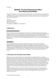
1. Introduction concerning the Scientific Method 7
Events of the material external world
Events of the inner psychological space
Can be described qantitatively
Two valued alternative logic (mathematics)
Can be described qualitatively
Multi-valued logic
Illustration 1: The two event–levels of the human world-experience
Die andere, hierzu konträre Richtung, sagt, es gibt diese psychischen Innenereignisse gar
nicht, es gibt überhaupt nur eine materielle Außenwelt, für die man auch
mitverantwortlich ist. Das ist die materialistische Schule. Aber ich meine, beide
Philosophien stellen eigentlich nur Eckpositionen dar, und ich finde es viel vernünftiger
zu sagen, ja, es gibt diese manifesten Ereignisse der physikalischen Außenwelt, wir lassen
aber auch die qualitativen virtuellen Ereignisse eines psychischen Geschehens zu. Ich
spreche hier gerne von zwei ganz verschiedenen Ereignisebenen.
The other, contrary approach, says that these psychological events do
not exist - there is only the external world in which we act. This is the
Materialistic school of thought. But I think both of these philosophies
only hit the edges of the truth. In my opinion, it is much more logical
to state that there are manifest events of a physical outer world. But
we must also permit the qualitative virtual events of psychological
occurences. I am satisfied to talk about two different levels of events.
Wenn wir nun aber irgendwelche Phänomene beschreiben wollen, müssen wir
berücksichtigen, dass wir Menschen in einer zweiwertigen vergleichenden Alternativlogik
denken, und dass der subtilste Aspekt dieser Logik das große Gedankengebäude der
Mathematik ist, mit dessen Hilfe wir quantifizierbare Dinge beschreiben und analysieren
können. Daher liegt der Gedanke sehr nahe, dass man auf diese quantifizierbaren
Ereignisse der materiellen Außenwelt die Metasprache der Mathematik anwendet um sie
zu beschreiben. Allerdings ist dieses für die Qualitäten des psychischen Erlebens nicht
möglich, denn Qualitäten lassen sich nicht quantifizieren. Mir scheint es daher sinnvoll zu
sein, zunächst diese Ebene virtueller Ereignisse eines psychischen Innenraums von der
Betrachtung auszuklammern und eine mathematische Beschreibung der Natur der
manifesten materiellen Ereignisstrukturen zu versuchen.
If we want to describe phenomena, we must consider that humans
think in a comparing, bi-valued alternative, true/false logic. That
logic finds its most subtle expression in the language of Mathematics,
with which we can describe and analyze measurable events. We have
therefore decided to use the meta-language of mathematics to
describe the quantizable events of the material external world.

8 1. Introduction concerning the Scientific Method
However, this is not possible for the qualities of psychological
experiences, since they do not lend themselves to quantification. It
seems necessary, then, to exclude all internal psychological virtual
events from our view, and its mathematical description, in order to
test our theories of manifest event structures in nature.
Die Gesamtheit aller dieser Ereignisse ist fixiert durch Quadrupel aus drei Ortsangaben
und einer Zeitangabe. Sie bilden also in ihrer Gesamtheit ein vierdimensionales
Kontinuum, ein Raum-Zeit-Kontinuum, in welchem sich alle physikalischen
Geschehnisse der materiellen Welt abspielen.
Wenn man nun Mathematik betreiben will und schließlich die Mathematik auf
irgendwelche physikalischen Gruppen von Phänomenen anwenden will um diese zu
beschreiben, muss man natürlich ein paar Voraussetzungen mitbringen. Beispielsweise
sagt man immer, Mathematik sei eine ganz nüchterne Wissenschaft, die sie zweifellos
auch ist – aber man braucht, um Mathematik zu betreiben, auch eine ganz gute Portion
Phantasie.
The totality of events is specified by a four-tuple containing three
spatial coordinates and a time. This totality forms a four-dimensional
continuum, a space-time continuum, in which all physical events of
the material world take place.
Now, if we want to use mathematics to describe a set of physical
events, this naturally brings with it a few conditions. For example,
one can say that mathematics is a completely rational science. It
certainly is. However, a good deal of imagination is needed as well.
Jeder von uns hat zum Beispiel versucht, irgendwelche Funktionen zu integrieren.
Keineswegs jede Funktion ist integrierbar, und wenn eine Funktion integrierbar ist, dann
ist es eine Frage, welche Transformation man findet, um sie integrierbar zu machen. Es
gibt aber keinerlei Kriterium und keinerlei Regeln, wie man die Transformation zu wählen
hat. Hier muss man sich aufs Fingerspitzengefühl verlassen. Wenn man aber für irgend
etwas Fingerspitzengefühl braucht – dann ist es eine Kunst, und gerade die Kunst des
Integrierens erfordert ziemlich viel Phantasie! Ein phantasieloser Mensch wird es nie
schaffen.
We have all tried to integrate functions, for example. Not all
functions are integrable. If it is not integrable, then it is a question of
finding a transformation that will make it integrable. But there are no
criteria and no rules to select the transformation. Here one must rely
on intuitive feeling. If one needs an intuitive feel for it – then it is an

1. Introduction concerning the Scientific Method 9
art, and the true art of integrating requires a good deal of fantasy!
Unimaginative people cannot do it.
Eine sehr nette Geschichte, die ich in Göttingen hörte, sagte, dass der bekannte
Mathematiker David Hilbert einen Schüler hatte, der sehr begabt war, der ihm aber weg
lief. Er wurde einmal gefragt, was denn aus diesem hoffnungsvollen jungen Mann
geworden sei, und da gab er zur Antwort: „Der ist Schriftsteller geworden. Für die
Mathematik hat er eben zu wenig Phantasie gehabt.“
Eine andere Eigenschaft, die man braucht, ist die der Intuition. Wenn ich die Mathematik
verwenden will um physikalische Sachverhalte zu beschreiben, muss ich zunächst einmal
intuitiv fühlen, in welcher Form man den Sachverhalt idealisiert, und welche empirische
Basis man auswählt. Vor allem braucht man unter Umständen sehr viel Talent und Gefühl,
um richtig zu approximieren. Die Kunst des Physikers ist die Kunst der richtigen
Approximation.
A nice little story, which I heard in Goettingen, was that the wellknown
mathematician David Hilbert had a very talented student, who
quit. When he was asked what had become of this promising young
man, he answered: “He became a writer. He did not have enough
imagination for Mathematics.”
One also needs intuition. If you want to use mathematics to describe
physical circumstances, you must first intuit the idealized
circumstances and select the basic empirical facts. Above all, you
need a lot of talent and feeling to approximate correctly. The art of
the physicist is the art of correct approximation.
Dann muss natürlich auch der Sinn für das Wesentliche eines Sachverhaltes ausgebildet
sein. Um einem Sachverhalt mathematisch zu formulieren, muss man sich immer wieder
klar werden über die Unerheblichkeit der Sinnfälligkeit. Man muss genau wissen, welche
Dinge wesentlich sind und wie man idealisiert, denn letzten Endes idealisieren wir immer
ein Modell, um das Wesentliche zu treffen.
Naturally, one must also be trained to sense what is relevant to the
circumstances. To formulate a mathematical model one must refine it
to remove insignificant details. One must know exactly which things
are relevant and as you modeled them. In the end, we always idealize
a model, in order to reflect what is relevant.

10 1. Introduction concerning the Scientific Method
Schließlich brauchen wir noch die Fähigkeit zur Abstraktion, das heißt, bei der
Beschreibung müssen wir versuchen, die Idee, die hinter dem Ding steht, zu erkennen und
den übergeordneten Zusammenhang zu erfahren.
Finally, we still need the ability for abstraction. That is, in building a
model we must try to see the idea behind the model, and to ultimately
understand the over-arching order of it.
Swan, ein englischer Physiker, der schon seit längerem verstorben ist, brachte einmal eine
nette Sache darüber, was passieren kann, wenn man diese eigentliche Fähigkeit zur
Abstraktion nicht mit bringt. Er erzählte eine nette Geschichte, die in der englischen
Kolonialzeit spielte. Man hatte damals in den britischen Kolonien in Afrika auch in den
entferntesten Buschdörfern kleine Schulen eingerichtet und irgendwelche, an sich ganz
wackeren Jägersleute eingesetzt, die nun Kinder unterrichten sollten und natürlich mehr
schlecht als recht ausgebildet waren. So ein Mann gab Geometrieunterricht. Er hatte
offensichtlich die Sache nicht so recht durchschaut und zeichnete eine Figur an die Tafel
mit einem rechten Winkel, der nach rechts offen war und sagte: „Merkt Euch, dass das ein
sogenannter rechter Winkel ist!“ Dann zeichnete er dieselbe Figur an die Tafel – aber jetzt
mit dem Winkel nach links offen und sagte: „Jetzt werdet Ihr mit Recht sagen, dass das
ein linker Winkel sei. Aber aus mir unbekannten Gründen ist das auf Befehl der britischen
Regierung auch ein rechter Winkel.“ Sie sehen, wie man unter Umständen daneben laufen
kann, wenn man diese Fähigkeit zur Abstraktion nicht besitzt.
Swan, an English physicist who died a long time ago, once nicely
described what can happen if one does not possess this sense of
abstraction. He told a story from the British colonial age. At that time
the British furnished small schools in the African bush, instructed by
native hunters, and the teachers were less than well trained. One such
man taught geometry.
Obviously he did not really understand his subject. He drew a figure
of a right angle on the board, open to the right, and said “This is a
right angle”. Then he drew the same figure on the board, but now
with the angle opening to the left, and said, “Now you may say with
good reason that this is a left angle. But for reasons unknown to me,
on the instructions of the British government, this is also a right
angle.” You see, you can get off track if you do not possess the ability
for abstraction.

1. Introduction concerning the Scientific Method 11
Wenn wir nun aber diese Voraussetzungen mitbringen und jetzt versuchen, irgendein
physikalisches System von zusammenhängenden Phänomenen mathematisch zu
beschreiben, dann können wir ja nicht auf irgendein voraussetzungsloses
Gedankengebäude aufbauen. Es kommt darauf an, bei der mathematischen Beschreibung
ein mathematisches Schema zu finden, das ein Analogon darstellt zu dem Phänomen oder
der Gruppe von Phänomenen, die wir beschreiben wollen, derart, dass dieses
mathematische Schema sämtliche quantitativ empirisch erfassten Seiten unseres Systems
von Phänomenen quantitativ richtig wiedergibt und eventuell auch Prognosen möglich
macht über Eigenschaften dieses Systems, die empirisch noch unbekannt sind.
But if we have the ability for abstraction, and if we now use these
ideas, and attempt to build a mathematical description of any
phenomenon or group of phenomena, we cannot start with some
unconnected thoughts.
We must find a mathematical description that is analogous to the
phenomenon or the group of phenomena we want to describe, in such
a way that this scheme correctly reflects all quantitatively described
aspects of our system of phenomena. Possibly, it also predicts
characteristics of this system, which are empirically still unknown.
Nun ist es natürlich so, dass wir nicht irgendein voraussetzungsloses mathematisches
Gebilde schaffen können. Wir können auch nicht von irgendwelchen mathematischen
Axiomen allein ausgehen. Wir brauchen Eigenschaften dieses phänomenologischen
Systems, dieses empirischen Systems von physikalischen Dingen, die wir zunächst
empirisch finden und als Basis benutzen. Das heißt, wir brauchen sozusagen einen
qualitativen empirischen Bahnhof für unsere intellektuelle Reise, von dem wir ausgehen
können, und gerade zur Auffindung eines geeigneten empirischen Ausgangssystems
braucht man die Eigenschaft der Intuition. Wir müssen praktisch einen Anker immer
wieder auswerfen und versuchen, wo er fasst, um dann anzusetzen. Dieses empirische
System sollte nach Möglichkeit sehr allgemeingültiger Art sein. Es sollte auf keinem Fall
irgendwelche Dinge erfassen, die eigentlich bereits in anderen Sätzen enthalten sind!
Now we can’t create a mathematical object unconditionally. Neither
can we proceed from axioms alone. We need characteristics of this
phenomenological system, this system of physical things, which act
as our qualitative empirical starting point for our intellectual journey.
To find such stations of suitable empirical output from our model, we
need intuition. We must in practise throw out our anchor over and
over, until it grabs something and we pull ourselves along. This
empirical system should use a universally valid approach. We should
avoid anchoring to anything which is already included in other
statements!

12 2. The deductive basis of the unified field theory
Wenn wir uns nun die Aufgabe stellen, die Welt, wie sie uns in Raum und Zeit erfahrbar
ist, diese physikalisch-materielle Welt, beschreiben zu wollen – die Ereignisebene der
virtuellen Ereignisse des psychischen Innenraums haben wir ausgeklammert – dann läuft
das schließlich darauf hinaus, das Wesen der Materie zu erfassen, also in einer möglichst
einheitlichen Form die Natur der Materie zu beschreiben, der Materie, die über
makroskopische Wirkungsfelder in physikalischen Zusammenhängen steht.
We now set ourselves the task of describing the physical world,
experienced by us in space and time. We have already excluded the
virtual events of our own interior psychology. Ultimately, this means
we have to extract the essence of it. We have to describe the physical
world mostly in a uniform fashion that is physically interconnected
by macroscopic fields of effects.
2. The deductive basis of the unified field theory
Elementarstrukturen, Volume 1
Chapter I – 1
Man muss sich sehr genau überlegen, von welcher empirischen Basis man ausgeht. Ich
hielt es für sinnvoll, überhaupt nur empirische Grundprinzipien der Natur zu verwenden,
die sich im gesamten von uns Menschen erfahrbaren physikalischen Bereich, immer
wieder bestätigt haben. Und zwar verwendete ich als Ausgangsbasis eigentlich nur drei
Prinzipien und die Tatsache, dass es Wirkungsfelder gibt, also eigentlich nur vier Sätze
(Axiome) und zwar:
a) die Erhaltungsprinzipien von Energie, Impuls und elektrischer Ladung,
b) gewisse Extremalprinzipien, die zum Beispiel das Prinzip des Entropieanstiegs
implizieren und mathematisch in der bekannten Weise durch Variationstheoreme
ausgedrückt werden können,
c) das Quantenprinzip, wonach bekanntlich eine Wirkung stets das ganzzahlige
Vielfache einer empirischen Naturkonstante, nämlich des Planck’schen
Wirkungsquants ist. Eine weitere Konsequenz wäre, dass die Materie atomistisch
strukturiert ist, das heißt, es gibt kein materielles Kontinuum und es gibt auch kein
energetisches Kontinuum – sondern es gibt Energiequanten und eine atomistische
Struktur der Materie.
d) die Tatsache, dass es makroskopisch wirkende Felder gibt, Felder des
Elektromagnetismus und der Gravitation, durch die makroskopische
Materiekonfigurationen in Zusammenhängen stehen.

2. The deductive basis of the unified field theory 13
Dabei verwende ich
d1) das elektromagnetische Induktionsgesetz in Form der Maxwell’schen Gleichungen,
die ebenfalls eine mathematische Verdichtung von elektrodynamischen Messreihen
sind,
d2) das empirische Newton’sche Gravitationsgesetz, das nur der mathematische Ausdruck
der drei Kepler’schen Gesetze ist, die wiederum eine Verdichtung der
lebenslänglichen Planetenbeobachtungen des Tycho Brahe darstellen.
We must be explicit about the empirical basis from which we start. I
think that it is important that we use only basic empirical principles
of nature which have been proven over and over in our experience. I
economized in using only three principles and the fact that there are
fields of interaction, which gives only four statements (axioms):
a) the conservation principles of energy, momentum and electrical
charge,
b) certain extremal principles, which imply the principle of
increasing entropy and can be expressed in the usual
mathematical way as variation theorems [calculus of variations],
c) the quantum principle, that is: an effect is always an integral
multiple of Planck’s constant, as we know. This also means that
the theory is discrete in structure, i.e. there are no material or
energy continua. Instead, there are quanta of energy and the
atomic structure of matter.
d) the fact that there are macroscopically operating fields of
electromagnetism and gravitation, which are connected by
macrosopic configurations of matter.
Specifically, I use:
d1) the electromagnetic induction law, in the form of Maxwell’s
equations, which are also a mathematical condensation of a
series of electro-dynamic measurements,
d2) Newton’s laws, which also represent a condensation of the life’s
work of Tycho Brahe in planetary observation.

14 2. The deductive basis of the unified field theory
Dabei muss natürlich unterstellt werden, dass diese empirischen Naturgesetze der
Gravitation und des Elektromagnetismus noch keineswegs als endgültig anzusprechen
sind, denn sie spiegeln doch nur die Empirie wieder – praktisch so wie beim Automaten,
aus dem, wenn man 10 Pfennig hineinsteckt, auch nur für 10 Pfennig Ware herauskommt.
Ich meine, was man in der Mathematik an empirischen Sachwerten hineinsteckt, kommt
bei einer solchen Formulierung auch wieder heraus – das heißt, diese Gesetze gelten nur
im Bereich ihrer Messgrenzen! Wir können zum Beispiel nicht erwarten, dass die
Maxwell-Gleichungen vollständig die Natur des elektromagnetischen Feldes wiedergeben.
Sie gelten eben nur in dem Bereich, in dem man elektromagnetische Messungen
durchführen kann. Das Newton’sche Gravitationsgesetz wird bestimmt sehr
korrekturbedürftig sein, wenn man die Wahrheit über das Phänomen Gravitation erfährt,
denn die Messtoleranzen bei der Bestimmung von Planetenbahnen sind doch ziemlich
groß.
In doing this, it must be considered that these empirical laws of
gravitation and electromagnetism must not be understood as
fundamental, since they only reflect experience. It is like a peanut
vending machine: if you put in a dime, you get only a dime’s worth
of peanuts. What you input as empirical values into a mathematical
formula is exactly what you get out, that is, these laws only apply
within the range that has been measured. We cannot expect, for
example, that the Maxwell equations express the complete nature of
the electromagnetic field. They apply only within the range in which
we can perform electromagnetic measurements. Newton’s
gravitational law certainly requires correction, if you understand the
truth about gravitation, since tolerances in the measurements of
planetary orbits are rather large.
Von diesen vier Grundsätzen ging ich aus. Und nun kann man in der bekannten Weise
zunächst einmal aus den Maxwell’schen Gleichungen des Induktionsgesetzes substituieren
und die vektoranalytischen Operator-Theoreme zur Umrechnung benutzen, wodurch man
zu einer transversalen Wellengleichung für sämtliche Bestimmungsstücke des
elektromagnetischen Feldes gelangt, bei der die Ausbreitungsgeschwindigkeit durch die
Naturkonstanten der Induktion und Influenz gegeben ist.
Man kann auf diese Weise die Lichtgeschwindigkeit sehr genau berechnen.
I started from these four principles. Now we can use a vector-analytic
approach to Maxwell’s equations to arrive at a transverse wave
equation for all components of the electromagnetic field data. The
propagation speed of this wave can be computed using the natural
constants of permitivity and magnetic permeability. One can compute
the speed of light very exactly this way.

2. The deductive basis of the unified field theory 15
Empirical starting point:
(empirically derived, well justified, quantitative physical statements of greatest possible universality)
Shurely there exist ...
a) Conservation laws
for:
b) Extremal principles:
(irreversible processes)
c) All effects are
quantized:
d) Material structures with
their exchange effects:
– Energy
– Momentum
– Charge
– Entropy-increase
(2. Main clause of the
thermodynamic theory)
→ no material or energy
continuum available
Within the macro range:
d1) Electromagnetic field
(Induction law)
d2) Gravitation (central field)
(Newton‘s gravitation
law), non covariant
Propagation of the electromagnetic induction in
empty charge free space as transverse waves
with c =
1
ε
0µ
0
In the micro realm:
d3) Exchange effects of
short range
Elektromagnetic relativity principle in R 4
(Lorentz invariant representation of electromagnetic
fields d1) of inertial reference systems moving
uniformly referred to each other) with
x4 = ict imaginary time dimension
(optical path)
$A − Lorentz group
Equivalence of energy and inertial mass
2
E = mc
Energy Mass
(inertia resistance)
Illustration 2: Empirical starting point
Man kann jetzt aufgrund der transversalen Wellengleichung auf das elektromagnetische
Relativitätsprinzip schließen und kommt von diesem Relativitätsprinzip zur Konstruktion
eines Minkowski-Raumes, das heißt eines vierdimensionalen Raumzeit-Kontinuums mit
drei reellen Dimensionen des kompakten physischen Raumes und der mit diesen
Dimensionen nicht vertauschbaren imaginären Lichtzeit.
You can move logically from the transverse wave equation to the
electromagnetic relativity principle, and from there to the
construction of a Minkowski space, i.e. a four-dimensional spacetime
continuum with three real dimensions of linear space and the
imaginary time dimension, [ict], that is not interchangeable with the
three real dimensions.

16 2. The deductive basis of the unified field theory
Dies führt schließlich zu einer Gruppe von Transformationen, bei der wir es mit
gleichberechtigten und konstant bewegten Inertialsystemen zu tun haben. Man erhält hier
die Lorentz-Gruppe, das heißt die Naturgesetze können jetzt in eine invariante Form
gebracht werden, deren Matrix bekanntlich die vierreihige Transformationsmatrix der
Lorentz-Gruppe ist. Es ist eine unitäre Matrix, mit der man nun die Naturgesetze
lorentzinvariant machen kann.
Eine Konsequenz dieser lorentzinvarianten Darstellung der Naturgesetze ist dann ein sehr
wichtiges Äquivalenzprinzip, nämlich das Äquivalenzprinzip zwischen Energie und
Trägheit. …
(Hier war das Tonband zu Ende. Es fehlt ein kurzes Stück. …)
This finally brings us to a group of transformations which we can
apply to inertial systems. Here you get the Lorentz group, i.e. the
laws of nature can be stated in an invariant form using a space-time
transformation matrix with four rows. It is a unitary matrix, with
which one can now make the laws of nature Lorentz invariant.
A consequence of this lorentz-invariant representation of the laws of
nature is a very important equivalence principle, i.e. the equivalence
principle between mass and inertia.
Diese beiden Äquivalenzprinzipien sind meiner Auffassung nach von fundamentaler
Bedeutung, jedoch kann man daraus alleine noch keine einheitliche Beschreibung der
Materie oder der Raum-Zeit-Welt aufbauen. Es sind auf diese Weise die spezielle und die
allgemeine Relativitätstheorie entstanden.
Schließlich wurde versucht, eine einheitliche Feldtheorie zu konstruieren. Es gibt zwar
sehr viele verschiedene Ansätze, jedoch sollte man nicht glauben, dass hier ein Anspruch
auf universale Gültigkeit gegeben ist, wenn man den wesentlichen Erfahrungsbereich (c),
nämlich das Quantenprinzip, ignoriert. Mir scheint es im Gegenteil so zu sein, dass eine
allgemeine Theorie des materiellen Geschehens letztlich nur eine Theorie der materiellen
Letzteinheiten sein kann, das heißt eine Theorie der elementaren Quanten eines
Materiefeldes!
These two equivalence principles are, in my view, of fundamental
importance. However, we cannot yet build a uniform description of
matter and space-time from this. This is how the special and general
theories of relativity were developed.
The final step was to design a unified field theory. Many attempts
were made. However, we should not believe in the universal validity
of this approach if we ignore the substantial experience of the

2. The deductive basis of the unified field theory 17
quantum principle c). I think the opposite – that a general theory of
material events can only be a theory of the ultimate elementary
quanta of matter, i.e. a theory of elementary quanta of a matter field!
Known elementary structures:
Ponderable material particles
Elementary particles with mass
Non-ponderable particles
(no rest mass)
Photons, (gravitons)
Non-ponderable particles
possess a field mass
c) All effects are
quantized:
→ No material or energetic
continuum exists
Superordinate term:
Matter field quantum Mq
Goal:
Unified description of the material world by a unified description of Mq, possibly by a structure
theory.
Requirement:
The spectrum of the ponderable elementary particles has to be derived accurately!
Illustration 3: The term of the matter field quantum
Ich habe hier den Begriff eines Materiefeldquants in meiner Arbeit geprägt, um einen
Oberbegriff zu haben. Ich verstehe darunter einmal die Quanten des elektromagnetischen
Feldes, die mit Lichtgeschwindigkeit fortschreiten, die sogenannten Photonen, denen nach
dem Energie-Materie-Äquivalent auch Trägheitsmasse zukommt, und ich verstehe
zugleich darunter die Gesamtheit der ponderablen, also wägbaren Letzteinheiten, die
empirisch als sogenannte Elementarteilchen bekannt sind.
Here, I coined the term “matter field quanta” as a generic term. On
the one hand it means quanta of the electromagnetic field, which
travel at the speed of light (photons). These have energy, and thus
inertial mass by the equivalence principle of energy and matter. On
the other hand, the same term describes the totality of ponderable
elementary quanta which we know as elementary particles.

18 2. The deductive basis of the unified field theory
Eine einheitliche Theorie der materiellen Welt kann nur eine einheitliche Theorie aller
dieser Materie-Feld-Quanten sein, wobei unter Umständen auch Quanten eines
Gravitationsfeldes denkbar wären, die man hypothetisch als Gravitonen bezeichnet.
Nun ist das Bild, das sich hier bietet, ungeheuer verwirrend. Es scheint überhaupt
aussichtslos zu sein, eine einheitliche Darstellung zu finden, denn die Eigenschaften, die
man beobachtet, sind außerordentlich widersprüchlich! Einerseits haben wir die
Feldquanten, die mit Lichtgeschwindigkeit fortschreiten und offensichtlich in ihrer
Struktur etwas völlig anderes darstellen als die Letzteinheiten der wägbaren Masse, der
Elementarteilchen. Hier haben wir eine ungeheure Fülle. Die Elementarteilchen
unterscheiden sich in drastischer Weise zum Beispiel in ihrer Existenzzeit. Es gibt sehr
labile und kurzlebige Partikel, also erlaubte Übergänge von freier Energie zu wägbarer
Substanz – als solche könnte man auch die Elementarteilchen bezeichnen – und wieder
andere, die eine entsprechend größere Lebensdauer haben, auch solche Elementarteilchen
wie Elektronen und Protonen, die eine unbegrenzte Lebensdauer haben, die stabil und
damit der Grund sind, dass es überhaupt Materie in unserem System gibt.
A unified theory of the material world can only be a unified theory of
all of these matter field quanta. The quanta of a gravitational field
might also be theoretically conceivable as the hypothetical graviton.
The picture that emerges is very confusing. There seems to be no
prospect of finding a uniform representation because the features we
observe are extraordinarily contradictory! On the one hand we have
the field quanta, which move at the speed of light, and differ in their
structure from those of ponderable mass, elementary particles, which
exist in a large variety of forms. The elementary particles themselves
differ greatly, for example, in their life spans. There are very unstable
and short-lived particles, which allow transitions from free energy to
ponderable mass, which is what we consider the elementary particles
to be. There are others, which are different in having a longer life
span. There are also elementary particles such as the electron and
proton, which have unlimited life spans, which are stable and
therefore the reason that matter exists in our world.
Elementarteilchen unterscheiden sich aber auch anders. Es gibt solche, die elektropositiv,
solche, die elektronegativ und solche, die elektrisch neutral sind. Die elektrisch geladenen
sind immer mit Elementarladungen versehen, das heißt auch das elektrische Ladungsfeld
ist kein Kontinuum – es gibt die elektrische Elementarladung, die sehr genau gemessen
werden kann, die man aber eigentlich in ihrem Wesen auch nicht so recht versteht.
Elementary particles differ in other ways, too. There are some that
are electrically positive, some negative and some which are
electrically neutral. The electrically charged ones always have

2. The deductive basis of the unified field theory 19
elementary charges, i.e. the electrical charge field is not a continuum.
There is an electrical elementary charge, which can be measured very
exactly, but its nature is still not understood.
Elementarteilchen haben die verschiedensten Massen. Sie unterscheiden sich sehr in ihren
Spin-Verhalten, sie haben offensichtlich so etwas ähnliches wie einen Drehimpuls, und
zwar sind diese Drehimpulse wieder ganzzahlige oder halbzahlige Vielfache des
Wirkungsquants. Es gibt zum Beispiel Partikel, die überhaupt keinen Drehimpuls haben,
deren Spinquantenzahl also Null ist. Dann haben wir die verschiedensten halbzahligen
Spinquantenzahlen, die sogenannte Fermionen beschreiben, die in ihrer Struktur wieder
etwas völlig anderes zu sein scheinen als die sogenannten Bosonen mit ganzzahliger
Spinquantenzahl. Man kann zum Beispiel Bosonen überlagern und dabei praktisch am
selben Ort die Amplituden gewissermaßen vergrößern! Aber bei Fermionen ist das nicht
möglich, hier scheinen sich „die Dinge im Raum zu stoßen“.
Elementary particles have more than different charges and masses.
They also differ in spin behavior, which is obviously similar to
angular momentum. Angular momentum is an integer or half-integer
multiple of a quantum effect. There are particles which are
completely missing an angular momentum, i.e. whose spin quantum
number is zero. Further, we have a variety of half-integer spin
quantum numbers, which describe Fermions. These seem completely
different in structure from the so-called Bosons, which have integer
spin quantum number. You can, for example, overlay Bosons
practically at the same place, and thus greatly increase their
amplitudes. But with fermions this is not possible – they seem to
have “something in space that pushes”.
Manche Elementarteilchen treten nur einzeln auf, andere wieder in ganzen Familie, die
verwand sind, in sogenannten Isospin-Multipletts, die auch wieder durch eine
Quantenzahl gekennzeichnet sind.
Wir haben dann beispielsweise Zerfallseigenschaften der Elementarteilchen, die alle nur
eine begrenzte Lebensdauer haben. Und hier kommt es zu den verschiedensten Zerfällen
und zu den verschiedensten Reaktionen, mit denen man experimentiert. Dafür ist nun
wieder eine Eigentümlichkeit gültig, die aus empirischen Gründen eingeführt wurde. Sie
unterscheiden sich in ihrer sogenannten Seltsamkeit, auch strangeness genannt.
Some elementary particles occur only individually, while others
occur in a whole related family of so-called isospin-multiplets. These
are also characterized by quantum numbers. There are also decay
characteristics – elementary particles usually have a limited life span.
Here we find, experimentally, the most diverse disintegrations and

20 2. The deductive basis of the unified field theory
reactions. There is a peculiarity that is responsible for this, that was
introduced for empirical reasons, and which we call Strangeness.
Kurz, ein außerordentlich verwirrendes Bild! Die Frage ist – wie kann man hier ein
Ordnungsprinzip hineinbringen? Man hat die verschiedensten Symmetrieuntersuchungen
angestellt, eine phänomenologische Klassifikation durchgeführt, aber ein einheitliches
Verständnis all dieser Strukturen ist nicht gelungen.
In short, this is an extraordinarily confusing picture! The question is
– how can one find an organizing principle here? An attempt was
made at a phenomenological classification, employing the most
diverse symmetry investigations, but a consistent understanding was
not achieved.
Ich meine, man muss hier nach Eigenschaften suchen, die allen diesen Partikeln
gleichermaßen zukommen, die bei keiner wie auch immer gearteten materiellen
Letzteinheit verschwinden. Ein Spin ist zum Beispiel nicht gut zu verwenden, denn es gibt
auch Partikel, bei denen er Null ist. Elektrische Ladungszahlen sind auch kein Kriterium,
denn es gibt neutrale Partikel. Aber eins ist für alle diese ponderablen Partikel, also für
solche die Ruhemasse haben, aber auch für die Photonen typisch, die imponderabler Natur
sind: Erstens haben alle eine von Null verschiedene Existenzzeit. Würde nämlich
irgendein Ding keine Existenzzeit haben, dann geschieht nichts, und wir könnten es
überhaupt nicht wahrnehmen! Es würde für uns nicht existieren.
Zweitens kommt all diesen Partikeln eine von Null verschiedene Masse zu, und zwar
entweder eine reine Feldmasse oder eine Ruhemasse. Auf keinen Fall ist aber diese Masse
gleich Null, denn wenn sie gleich Null wäre, würde das Ding nicht existieren, auch wenn
es eben nur freie Feldmasse ist, wie beim Photon!
So I conclude that we must look for one characteristic that these
particles share, which does not disappear for any fundamental
elementary unit, whatever it may be. Spin is not a good example
because there are particles with zero spin. Electrical charge is also not
a good criterion, because there are neutral particles. There is one
property of all these ponderable particles, which imponderable
photons also share: they have a lifetime different from zero. If
anything has no lifetime, then nothing happens, and we would not
notice its imprint on the world. It would not exist.
Secondly, all particles have a mass different from zero, either a pure
field mass or a rest mass. None have a mass of zero, because if it
were identically zero, the thing would not exist. Even the photon has
a free field mass.

2. The deductive basis of the unified field theory 21
Von den Existenzzeiten auszugehen schien mir nicht sehr attraktiv zu sein. Ich fand auch
gar keinen vernünftigen Anlass. Aber man könnte von der Tatsache ausgehen, dass alle
diese Partikel Massen oder Energiemassen sind. Es sind eben erlaubte Übergänge von
freier Energie zu wägbarer Materie.
Nun gibt es dieses Äquivalenzprinzip zwischen Trägheit und Gravitation, und das wäre
die allgemeine Gravitation, die zugleich auch das allgemeine Hintergrundphänomen für
die gesamte Fülle möglicher materieller Letzteinheiten zu sein scheint.
It did not seem very attractive to me to begin with the existence times
and I’ve found no obvious reason to do so. But we could start with
the fact that all of these particles have masses or an energy massequivalent.
They are just transitions from free energy into ponderable
mass.
Now we can apply the equivalence principle between inertia and
gravitation to say that inertia and gravitation are the same thing. It is
also the same thing as the general background for all fundamental
matter field quanta.

22 3. Formulation of an invariant Gravitation theory
3. Formulation of an invariant Gravitation theory
Elementarstrukturen, Volume 1
Chapter I – 2
Leider wissen wir gerade über dieses Phänomen der Gravitation nur sehr wenig, denn das
Newton’sche Gravitationsgesetz gilt bestimmt nicht hier. Wir kennen auch nicht den
Verlauf des Gravitationsfeldes beispielsweise in der unmittelbaren Nachbarschaft eines
Elementarteilchens! Aber wir können indirekt doch einiges sagen. Wir können zum
Beispiel sagen, dass die Gravitation offensichtlich ein Zustand ist, der sich vom Nichts
deutlich unterscheidet.
Wenn überhaupt etwas existieren oder aufgebaut werden soll, dann braucht man dazu
Energie. Energie und träge Masse, die wiederum Quelle einer Gravitationswirkung sein
kann, sind äquivalent! Andererseits scheint das Gravitationsfeld selber, bezogen auf die
felderregende Masse, additiver Natur zu sein. Mir fällt es offen gesagt schwer,
anzunehmen, dass zwar die Materie insgesamt ein Gravitationsfeld verursacht, dass ihre
letzten Bausteine aber keines haben sollen. Es scheint mir so zu sein, dass, wenn es
Quanten der Materie gibt, diese Quanten zumindest elementare Gravitationsfelder
definieren.
Unfortunately we truly know very little about the phenomena of
gravitation, because Newton’s gravitation law certainly does not
apply here. We do not know how the gravitational field works in the
immediate neighborhood of an elementary particle! But we can draw
some conclusions nevertheless. We can say, for instance, that
gravitation is obviously a condition that differs from nothing.
If anything is to exist or be created, then one also needs energy.
Energy and inertial mass, which again can be the source of a
gravitational effect, are equivalent! On the other hand, the
gravitational field itself seems to be of an additive nature, related to
the field inertia. I can hardly imagine that matter, which causes the
gravitational field, should have no gravitational effect from its
fundamental constituents. It seems more likely that, if there are
elementary quanta of matter, then these quanta define elementary
gravitational fields.

3. Formulation of an invariant Gravitation theory 23
Ob das Gravitationsfeld nun selber ein Quantenfeld ist, wissen wir nicht. Aber aus
logischen Gründen würde ich es rein hypothetisch unterstellen, denn typisch für ein
Quantenfeld ist die Unschärferelation, wonach wir gewisse Größen, zum Beispiel Ort und
Bewegung, Energie und Zeit, also kanonisch konjugierte Größen, nicht gleichzeitig exakt
messen können. Wir machen grundsätzliche Fehler, und zwar ist das Produkt dieser Fehler
mindestens gleich dem Planck’schen Wirkungsquant.
Wenn ich einmal unterstelle, dass wir irgendeine Kraftwirkung haben, die zwei Dinge in
Zusammenhang setzt, dann gilt diese Unschärferelation! Wenn diese Kraftwirkung jetzt
durch eine bloße Gravitationswirkung ersetzt wird, so fällt es mir offen gesagt etwas
schwer anzunehmen, dass ich plötzlich die beiden Größen beliebig genau messen kann.
Dieser Gedanke stammt von Bondy und ich habe den Eindruck, dass man auf diese Weise
wohl zunächst hypothetisch unterstellen kann, dass wir es bei der Gravitation auch mit
einem quantisierten Feld zu tun haben, obwohl wir nicht wissen, wie diese Quantisierung
eigentlich zustande kommen kann.
Now we do not know if the gravitational field is a quantum field, but
for argument’s sake, let’s assume that it is. The uncertainty principle
typically holds for a quantum field, so we are unable to
simultaneously measure certain conjugate pairs. For example,
position and momentum, energy and time. We find a fundamental
uncertainty at least as large as Planck’s quantum effect.
If I assume that we have an interaction force which connects two
things, then this uncertainty relation applies! If a bare gravitational
effect is substituted for this interaction force, then it seems difficult to
imagine that I can suddenly measure both conjugate attributes
exactly. This idea comes from Bondy. I think that we must assume
gravitation is also a quantized field, although we do not know how
this quantization comes about yet.
Nun schien es mir vernünftig zu sein, mich zunächst einmal ganz allgemein – und zwar
ohne jetzt an den Mikrobereich der Welt zu denken – etwas konkreter mit den Phänomen
der Gravitation zu befassen. Wir wissen zwar wenig von der Gravitation, aber ich kann
zum Beispiel das Newton’sche Gravitationsgesetz in die Poisson’sche Fassung eines
Quellenfeldes bringen. Man hat einen Feldvektor, der hier als Beschleunigung auftritt und
im statischen Fall der Gradient einer skalaren Ortsfunktion ist. Die Divergenz des
Feldvektors ist dann proportional zur Dichte der felderregenden Masse.
Now it seemed reasonable, without getting too detailed about the
microscopic range of the world, to think more concretely about the
phenomenon of gravitation. We know little of gravitation, but we can,
for example, bring Newton’s gravitation law into Poisson’s version of
a source field. We have a field vector, which is acceleration. In the

24 3. Formulation of an invariant Gravitation theory
static case, it is the gradient of a scalar position function. The
divergence of the field vector is then proportional to the density of
the field-source mass.
Man könnte überlegen, was geschieht, wenn eine zeitliche Variabilität zugelassen wird.
Ich gehe also jetzt zum Beispiel von einer Massenverteilung aus, die nicht homogen ist,
die irgendwelche Inhomogenitäten oder Anisotropien hat, und die sich zugleich zeitlich
verändert, so dass eine partielle Zeitableitung der Massendichte der Feldquelle existiert.
Ich lasse nicht zu, dass bei dieser zeitlichen Veränderung irgendwelche Materie eine
bestimmte geschlossene Fläche, die diese Materie umschließt, verlässt, und betrachte jetzt
das Gravitationsfeld praktisch von außen.
Man kann so auf rein logischem Wege das Newton’sche Gravitationsgesetz erweitern und
zwar für den Fall, dass es solche zeitliche Änderungen gibt, und dabei auch die Feldmasse
mit berücksichtigen.
Dann würde zwischen unserem jeweiligen Beobachtungspunkt und der felderregendem
Masse auch Gravitationsfeldmasse liegen, die ihrerseits auch wieder Gravitation
verursachen kann, so dass der Verlauf des Feldes hier in einer unbekannten Weise noch
verändert wird – natürlich weit unter jeder Messbarkeitsschranke!
Let us consider what happens if we introduce a temporal variability.
We start with a mass distribution which is not smooth, which has
inhomogeneities or anisotropies, and which varies in time so that a
partial time derivative of the mass density of the field source exists.
We do not allow the source to leave a certain closed surface, which
surrounds the source. Now consider the gravitational field outside of
the surface.
One can logically extend Newton’s gravitation in this way if these
temporal changes exist and we consider a field’s mass.
Then between our point of observation, and the field-generating
mass, there is also the gravitational field’s mass, which has its own
gravitational effect, so that the form of the field is changed in an
unknown manner and so on down to the limits of measurability!

3. Formulation of an invariant Gravitation theory 25
Illustration 4: Mass and field masses in the dynamic view of
gravitation
Zeitlich veränderliche Gravitationsfelder lassen sich nun beschreiben, wobei man
zunächst einmal zur Aussage kommt, dass sich eine Störung des Gravitationsfeldes mit
einer bestimmten Geschwindigkeit ausbreitet, die weder Null noch unendlich, sondern
eine von 0 verschiedene Zahl ist.
Temporally variable gravitation fields can now be described. First we
come to the conclusion that a disturbance of the gravitational field
spreads with a certain speed which is a finite number different from
zero.

26 3. Formulation of an invariant Gravitation theory
Man hat einmal gesagt, es sei die Lichtgeschwindigkeit. Es kann sein, dass es die
Lichtgeschwindigkeit ist, aber ich finde, man sollte diese Frage einfach offen lassen. Man
sollte sich damit zufrieden geben, dass es irgendeine Geschwindigkeit sein kann, und sich
hier nicht spekulativ von vornherein auf die Lichtgeschwindigkeit festlegen.
Man lässt hier am besten die Frage nach der Ausbreitungsgeschwindigkeit von
Gravitationsstörungen offen und beschreibt nun das sich zeitlich ändernde
Gravitationsfeld in einer reellen Raumzeit, und zwar benutzt man hier nicht den üblichen
Minkowski-Raum, sondern zunächst einmal aufgrund des Zeitverhaltens des
Gravitationsfeldes eine reelle Zeitkoordinate.
Diese Raumzeit ist natürlich nicht die wirkliche Raumzeitwelt, denn sie gilt nur unter der
Voraussetzung, dass nur solche Gravitationsfeldvorgänge existieren, die sich zeitlich
verändern, ohne dass eine wirkliche Feldquelle vorhanden ist!
You might guess that it is the speed of light. It might be that it IS the
speed of light, but I think we should simply leave this question open.
We should content ourselves that it can be any speed, and not
speculatively commit ourselves from the start.
It is best to leave open the question of the speed of propagation of
gravitational disturbances at this point. Now we describe the
temporally changing gravitational field in a real space-time. We do
not use the usual Minkowski space, but one with a real time
coordinate, because of the temporal behaviour of the gravitational
field.
This space-time is naturally not the real space-time we see, because it
was derived under the condition that only such temporally changing
gravitational effects exist, but no real field source is present!
Man kommt bei dieser Beschreibung nun zu einer Darstellung in vier reellen
Dimensionen. Es lässt sich hier auch ein vierreihiger Feldtensor definieren, der aus
Gravitationsfeldgrößen aufgebaut ist, und man kommt auch zu einer Lorentzgruppe, deren
Matrix jetzt aber nicht unitär sondern orthogonal ist. (Ich bezeichne grundsätzlich eine
Matrix mit orthogonalen Eigenschaften über dem reellen Zahlenkörper als „orthogonal“.
Sind die Elemente aber komplexe Zahlen, bezeichne ich sie als „unitär“. Es erweist sich,
dass diese begriffliche Verfeinerung auch in der Physik eigentlich recht gut zu verwenden
ist.)
Doing this, we arrive at a model with four real dimensions. We also
can define a field tensor with four rows composed of gravitational
field values. We also have a Lorentz group, whose matrix is not,
however, unitary, but orthogonal. (In principle, I call a matrix with

3. Formulation of an invariant Gravitation theory 27
orthogonal characteristics over the real number field “orthogonal”.
If the elements are complex numbers instead, I call it “unitary-like”.
I find that this conceptual refinement is actually very useful in
physics generally.)
Es ergibt sich hier, wie gesagt, eine Tensordarstellung des Gravitationsfeldes in dieser
Hilfskonstruktion einer reellen Raumzeit. Jetzt kann man in der bekannten Weise aus dem
elektromagnetischen Induktionsgesetz ebenfalls eine Tensordarstellung gewinnen; und
zwar in einer Minkowski-Welt, mit einer imaginären Zeitkoordinate – wenn wir
Gravitationsvorgänge nicht berücksichtigen.
Nun, beide Raumzeiten scheinen nur Hilfskonstruktionen zu sein. Die wahre Welt ist es
nicht, denn in der wirklichen Welt haben wir sowohl elektromagnetische als auch
gravitative Vorgänge, oder wir haben materielle Feldquellen, die ein Gravitationsfeld
erregen. Es gibt keine Masse ohne Gravitation, und wir haben auch keine Gravitation
ohne Masse!
Diese beiden Hilfskonstruktionen scheinen mir nur tangentiale Raumzeiten der wahren
Raumzeit zu sein, derart, dass die tatsächlichen Größen, mit denen wir es in der
materiellen Natur zu tun haben, praktisch sowohl in der einen wie auch in der anderen
Raumzeit definiert sind, und diese Verschränkung ist das, was wir eigentlich Raumzeit
nennen können.
As we said, we get a tensor representation of the gravitational field in
this auxiliary construction of a real space-time. Now we can likewise
get a tensor representation in the usual way known from the
electromagnetic induction law, specifically in a Minkowski space
with an imaginary time coordinate – if we do not consider gravitation
effects.
Now both space-times seem to be only auxiliary constructions. The
real world is like neither. In the real world we have both
electromagnetic and gravitational effects. We also have material
sources generating a gravitational field. There is no mass without
gravitation, and we have no gravitation without mass either!
Both auxiliary constructions seem to me to be only tangential spacetimes
to the true space-time. Actual measurements in nature are
practically defined in both space-times, and the intersection is what
we might call real space-time.

28 3. Formulation of an invariant Gravitation theory
Einstein
Electromagnetic Lorentz
transformation in R −4
$A −
x ict
− 4
=
Electromagnetic field tensor
F km
( R )
−4
Heim
Gravitational Lorentz
transformation in R +4
$A +
x+ 4
= ω t when β > 0
x− 4
= iω t when β < 0
General Lorentz
transformation in R 4
x
4 =
B$ A$ A$
ict
=
+ −
Uniform field tensor
in R 4 (Minkowski-space)
M km
Invariance
approximately B
( R )
4
Gravitation field tensor
G km
( R )
+4
Illustration 5: Construction of a uniform field description
Nun zeigt zunächst einmal eine geometrische Betrachtung, dass in dieser tatsächlichen
Raumzeit auch die Zeitkoordinate eine imaginäre Lichtzeit ist. Das heißt, es ist auch ein
Minkowski-Raum, denn werden die beiden Lorentzmatrizen multipliziert, also die
orthogonale Matrix der Gravitationswelt und die unitäre des elektromagnetischem
Relativitätsprinzips, dann zeigt sich erwartungsgemäß, dass der Kommutator des
Matrixprodukts die Nullmatrix ist, das heißt die Multiplikation ist kommutativer Art.
Jetzt wird deutlich, dass die Ausbreitungsgeschwindigkeit gravitativer Feldstörungen
überhaupt keinen Einfluss auf die Begrenzung der Geschwindigkeit materieller Körper
durch die Lichtgeschwindigkeit haben kann, denn in den Elementen der Einstein’schen
Lorentzmatrix treten Gravitationsgrößen nur als Korrekturfaktoren auf, die aber praktisch
vom Wert 1 nicht abweichen. Es ist eigentlich so, dass eine mögliche Abweichung – ich
habe mir das ziemlich gründlich auch quantitativ überlegt – praktisch unter jeder
Messbarkeitsschranke heutiger Möglichkeiten liegt, so dass sie empirisch nicht in
Erscheinung tritt.

3. Formulation of an invariant Gravitation theory 29
A purely geometrical view shows that in this actual space-time, the
time coordinate is also an imaginary one. That is, it is also a
Minkowski space, because when we multiply the orthogonal matrix
of gravitation and the unitary matrix of the electromagnetic relativity
principle, then we get, as expected, the zero-matrix as the
commutator of the matrix product. That is, the multiplication is
commutative.
It is now clear that the propagation speed of gravitational field
disturbances can have no influence on the speed of material bodies
being limited by the speed of light. Because in Einstein’s Lorentz
matrix, gravitational measurements appear only as correction factors,
which do not deviate substantially from 1. It is actually true that any
deviation is practically unmeasurable with today’s techniques, so that
it goes unnoticed in practice. (I considered this quite thoroughly in
quantitative terms).

30 4. Unified field description
4. Unified field description
Elementarstrukturen, Volume 1
Chapter I – 3
Die Raumzeitvorgänge gravitativer und elektromagnetischer Art bezog ich nun
gemeinsam auf eine solche Minkowski-Welt, das heißt auf eine Raumzeit mit imaginärer
Zeitkoordinate. Es schien nun, um diese Beschreibung durchzuführen, sinnvoll zu sein,
die gewonnenen Feldtensoren zu einem einheitlichen Feldtensor zu kombinieren, der
sowohl die elektromagnetischen als auch die gravitativen Feldgrößen enthält.
Leider war hier das Problem vieldeutig, denn man müsste jetzt von diesen Feldtensoren
die Vektordivergenz im Minkowski-Raum bilden. Diese Vektordivergenz wäre dann einer
Art Viererstrom proportional, der aus einem Materiefluss und einem elektrischen
Ladungsfluss besteht. Aber diese Vieldeutigkeit der Kombination der Feldtensoren zu
einem einheitlichen Feldtensor des elektromagnetisch-gravitativen Feldes reduziert sich
auf eine Zweideutigkeit, denn man muss fordern, dass sich die bekannten empirischen
Gesetze der Gravitation und der Maxwellgleichungen als Sonderfälle ergeben, wenn man
die eine oder andere Gruppe von Größen streicht.
I combined the gravitational and electromagnetic space-time effects
together into a Minkowski space, i.e. to a space-time with an
imaginary time coordinate. It seemed to be meaningful to combine
these two field tensors into a unified field tensor, which contains both
electromagnetic and gravitational field components.
Unfortunately, at this point, there was an ambiguity because one had
to form the vector divergence in Minkowski space from these field
tensors. This vector divergence would then be a four-vector,
consisting of a matter flux and an electrical charge flux. But this
ambiguity of the combination of the field tensors to a unified
electromagnetic-gravitational field tensor reduces to only two
possibilities because we must demand that the well-known laws of
gravitation and the Maxwell equations result as special cases in the
limit of zero electromagnetic effects or zero gravitation respectively.

4. Unified field description 31
Wenn man diesen Anschluss an die vorhandene Empirie fordert – und den müssen wir
fordern, sonst ist die Theorie ganz einfach falsch – dann reduziert sich die Vieldeutigkeit
auf eine Zweideutigkeit.
Nun muss man beide Wege durcharbeiten und kann dann den einen Weg ad absurdum
führen. Dieser ist wohl eine mathematisch logische Möglichkeit, die aber in der Natur
nicht verwirklicht ist. Denn würde dieser eine Weg der Natur entsprechen, dann würden
sich Aussagen über makroskopische Vorgänge ergeben, die in drastischster Weise
erscheinen müssten, die aber tatsächlich niemals nachweisbar sind, während sich der
andere Weg vollständig in die bekannte Empirie einpasst.
So sah ich mich veranlasst, diesen einen Weg weiter zu verfolgen. Wenn ich nun
unterstelle, dass wir auf diese Weise einen einheitlichen Feldtensor erhalten haben – dann
kann man hieraus auch einen einheitlichen Energiedichte-Tensor formulieren, und zwar in
der bekannten Weise durch eine Iteration des Feldtensors f ik , das heißt man multipliziert
i
in
diesen Tensor tensoriell mit sich selbst und bildet das Matrizenspektrum T
k
= f
kn
f .
Man erhält dann einen Energiedichtetensor T ik , der nun aber die Energiedichte eines
einheitlichen Feldes darstellt, nämlich einer Feldquelle mit ihrem Gravitationsfeld. Dies
erscheint nun als Einheit, und darauf muss es jetzt ankommen.
If we insist on this connection to existing experience – and we must
demand that or the theory is simply wrong – then the ambiguity
reduces to only two possibilities.
We must now follow both paths of the ambiguity to see if either
results in a reductio ad absurdum. This would be a mathematically
logical deduction, which is not, however, seen in nature. If that one
path would correspond to nature it would lead to statements about
macroscopic effects which should definitely be clearly observable,
but which are never observed. The other path would fit completely
with our experience.
Therefore I was compelled to follow this chain of reasoning a bit
further. If I now assume that we have derived a unified field tensor in
this way, then we can also formulate a unified energy density tensor,
in the usual way – by an iteration of the field tensor f ik
. We multiply
this tensor by itself tensorally then it forms a spectral matrix
i
in
T
k
= f
kn
f . We then have an energy density tensor T ik
representing the
energy density of a combined field, that is: a field source with its
gravitational field. It is a unified field, which is what we need.

32 4. Unified field description
Man kann im elektromagnetischen Fall diesen Energiedichtetensor explizit ausdrücken.
Da aber das Energie-Materie-Äquivalent gilt, das ja jeder Energie auch träge Masse
zuordnet, kann man natürlich diesen nichtsymmetrischen, oder hier besser
nichthermiteschen, Energiedichtetensor gut verallgemeinern.
Zum Begriff hermitesch und symmetrisch: Auch hier habe ich die Unterscheidung
gemacht, die in der Mathematik zwischen reellen und komplexen Zahlen üblich ist. Ein
Tensor, dessen Komponenten reelle Zahlen sind, und dessen Indizierungen vertauschbar
sind, nennen wir bekanntlich symmetrisch.
Handelt es sich aber um Komponenten, die aus komplexen Zahlen bestehen, müsste man
immer bei der Transposition der Indizierung zugleich eine komplexe Konjugation
durchführen. Solche Tensoren, wenn sie auch symmetrisch erscheinen, bezeichnen wir als
hermitesche Tensoren.
Der allgemeine Energiedichtetensor erscheint aber nichthermitesch, was an der
Wechselbeziehung zwischen Gravitation und ihrer Feldquelle liegt. Er lässt sich im
elektromagnetischen Fall folgendermaßen schreiben:
We can express this energy density tensor explicitly in the
electromagnetic case. However, since the energy-matter equivalence
assigns an inertial mass to each energy, one can naturally generalize
this non-symmetrical or more correctly, non-Hermitian, energy
density tensor here as well.
Regarding the terms Hermitian and symmetric: I make the distinction
here between real and complex numbers, as is usual in mathematics.
A tensor whose components are real numbers, and whose indices are
interchangeable we call symmetric.
If it contains components which consist of complex numbers, we
would also have to do a complex conjugation at the same time as the
index transposition. I call such tensors Hermitian, even if they are
symmetric and real.
The general energy density tensor seems to be non-Hermitian
however, because of the interaction between gravitation and its field
source. For the electromagnetic case alone, it can be written as
follows:
T
= W
+ Φ
W
( E)
ik ik ik
,
ik ki ik
= W ≈ V
(1)

4. Unified field description 33
(E)
Ich habe den einheitlichen Energiedichtetensor mit T
ik
bezeichnet, wobei die
Indizierungen die Dimensionen in Raum und Zeit angeben. Im Fall des
elektromagnetischen Feldes ist der einheitliche Energiedichtetensor mit hochgestelltem
*
Suffix E gekennzeichnet. Er baut sich aus einem hermiteschen Anteil W ik
= W ki i und
einem antihermiteschen Anteil Φ
ik
auf, wobei der hermitesche Anteil in sehr guter
Näherung mit dem sich unter Vernachlässigung der Gravitation aus der Maxwelltheorie
ergebenden kanonischen Energiedichtetensor V ik identisch ist. Er entsteht sogar aus
diesem Tensor, wenn die Gravitationsfeldgrößen überhaupt gestrichen werden.
Der antihermitesche Anteil wird durch seine Komponenten
Vektorprodukt, Gl. (2), aufgebaut
Φ
ik
aus einem
(E)
I have also designated the energy density tensor as T
ik
, where the
indices indicate the dimensions in space and time. In the case of the
Electromagnetic field, the unified energy density tensor is indicated
*
by the upper index E. It is composed of a Hermitian portion W ik
= W ki
and a non-Hermitian portion Φ ik
. The Hermitian portion is a very
good approximation to the Maxwell theory canonical energy density
tensor V
ik
, ignoring gravitation. In fact, it is the limit of this tensor, as
the Gravitational field goes to zero.
The non-Hermitian portion has components
cross product, EQ. (2)
Φ ik
developed from a
Φ
ik
= −Φ ki
;
12
= ϕ3
r r ⎛ r r µ ⎞
⎜
0
ϕ ~ g ×
⎟
E + H
⎝ ε
0 ⎠
Φ ; Φ
13
= −ϕ
2
, Φ
23
= ϕ1; Φ
j , 4
= −ϕ
j
(2)
In diesem Vektorprodukt ist g r ein Gravitationsfeldvektor, während E r und H r die
elektrische bzw. magnetische Komponente des elektromagnetischen Feldes darstellt. Die
µ
0
Quadratwurzel ist bekanntlich auch eine Naturkonstante, und zwar der
ε
0
elektromagnetische Wellenwiderstand des Leerraumes.
In this vector product g is a gravitational field vector, while E and H
represent the electrical and magnetic component respectively of the
electromagnetic field.

34 4. Unified field description
The square root
µ
0
ε
0
is well known as a natural constant, the
electromagnetic characteristic impedance of empty space.
Natürlich kann man den nichthermiteschen Tensor Tik
≠ Tki
auf eine allgemeine Masse,
die ein Gravitationsfeld erregt, erweitern. Wenn man nun das Gravitationsfeld im Tensor
streicht, so erreicht man, wie aus Gl. (3) ersichtlich, wenn der Gravitationsvektor
… (3)
gleich Null gesetzt und die Nichthermitezität aufgegeben wird, den rein hermiteschen
Tensor V ik des elektromagnetischen Feldes, wie er aus der klassischen Elektrodynamik
bekannt ist.
Naturally one knows the non-Hermitian tensor Tik
≠ Tki
extends to a
general mass, which excites a gravitational field. If the gravitation
vector is directly set to zero and the non-Hermetiticy is given up, then
one reaches the purely Hermitian tensor V ik
of the electromagnetic
field, as EQ. (3) shows, and as classical electrodynamics confirms:
T
ik
r
*
( g = 0 r
) = V = V ki
ik
(3)
k
Vi
kl 1 k mn
= f f
il
− δ
i
f mn
f
(4)
4
Jetzt muss allerdings das von ihm erregte Gravitationsfeld anders beschrieben werden.
Das ist bekanntlich in der allgemeinen Relativitätstheorie gemacht worden, wo man
sämtliche ein-eindeutigen stetigen Koordinatentransformationen betrachtet und daraus
eine homogen quadratische Differentialform der Metrik gebildet hat. (Wenn man von den
geodätischen Koordinaten auf irgendwelche, zum Beispiel kartesische Koordinaten,
transformiert, stehen vor quadratischen Gliedern die Komponenten des sogenannten
metrischen Fundamentaltensors g ik = g ki , die ihrerseits wieder Funktionen der
Raumzeitkoordinaten sind.) Der Fundamentaltensor liefert im hermiteschen Fall eine
Riemann-Geometrie.
Now, however, the gravitational field excited by it must be described
differently. As we know, that is done in general relativity theory,
where one considers curvilinear coordinate transformations to form a
homogeneous square differential form of the metric. (If we transform
into any general coordinates, such as cartesian coordinates, then
component elements of the metric fundamental tensor g
ik
= gki
appear
before square components (which again are functions of the space-

4. Unified field description 35
time coordinates). The fundamental tensor provides Riemannian
geometry in the Hermitian case.
Unified field tensor
in R 4
(Minkowski-space)
M km
( R )
4
Iteration
(tensorial multiplication
with itself and formation
of the spectral matrix)
Uniform energy impulse density tensor
(phenomenological matter tensor)
T = M M
T
ik
ik
4
∑
m=
1
im
mk
= T
+ −
+ T ik
ik
hermitian
in the electromagnetic case
T
( E )
ik
= W +Φ
ik
ik
antihermitian
T
ik
V
No gravitation
r r r
p = $ G , µ = 0
( )
=
ik
Maxwell canonical
energy density tensor
Illustration 6: The general energy density tensor

36 4. Unified field description
Man kann eine Parallelverschiebung in einem solchen nichteuklidischen Raum betrachten,
in dem der Fundamentaltensor vom Einheitstensor verschieden ist, und kommt dabei zu
den sogenannten Christoffel-Symbolen, Gl. (5), die in der bekannten Weise durch partielle
Ableitungen des Fundamentaltensors definiert sind.
Considering a parallel transport in such a non-Euclidean space, in
which the fundamental tensor is different from the unit tensor, we
find the Christoffel symbols, EQ. (5), which are defined as usual by
partial derivatives of the fundamental tensor.
⎧ i ⎫ ⎧ i ⎫ ⎛ ∂ ∂ ∂ ⎞
⎨ ⎬=
⎨ ⎬ =
1 im g
km
g
ml
g
kl
g ⎜ + − ⎟
(5)
l k m
⎩kl⎭
⎩lk⎭
2 ⎝ ∂x
∂x
∂x
⎠
Die beiden kovarianten Indizierungen stehen unten, die kontravarianten oben. Sie sind in
ihren kovarianten Indizierungen hermitesch.
Man kann nun den metrischen Fundamentaltensor als tensorielles Gravitationspotential
interpretieren, weil die Geodätengleichung Gl. (6) gilt, die durch die Christoffel-Symbole
ausgedrückt werden kann.
The two lower indices are covariant, the upper indices are
contravariant. These symbols are Hermitian in their covariant indices.
We can now interpret the fundamental metric tensor as a tensorial
gravitational potential, because the geodesic equation EQ. (6) applies,
which can be expressed by the Christoffel symbols.
i
&& x
⎧ i ⎫ k
+ ⎨ ⎬x&
x&
⎩kl⎭
l
= 0
(6)
Einsteins Überlegung war nun die, dass das Prinzip (a) unserer empirischen Basis, also
das Energieerhaltungsprinzip, gelten muss. Das heißt, dass die Vektordivergenz des
Energiedichte-Tensors, beispielsweise hier des elektromagnetischen Energiedichte-
Tensors V ik , verschwinden muss. Der Tensor ist divergenzfrei, das heißt die
Vektordivergenz ist gleich dem Nullvektor:
Einstein’s thought was that now the energy conservation principle
(principle a) of our empirical basis) must apply. That is, that the
vector divergence of the energy density tensor must disappear – for
example the electromagnetic energy density tensor V ik
. The tensor is
divergence-free, that is, the vector divergence is equal to the zerovector:

4. Unified field description 37
ik
T ; k = 0
(7)
(Tonband zu Ende, es fehlt hier ein kurzes Stück. …)
So entstehen nun die Grundgleichungen der allgemeinen Relativitätstheorie Gl. (8), die so
zu interpretieren sind: Wir haben einen phänomenologischen Materie-Tensor proportional
gesetzt einem reinen Struktur-Tensor, und nun deutet man diesen Struktur-Tensor als
Gravitation.
So now the equations of General Relativity produce EQ. (8), which
are to be interpreted thus: we have a phenomenological matter-tensor
proportional to a pure structure tensor, and now this structure tensor
is interpreted as gravitation.
1
R
ik
− g
ik
R ~ V
2
k
R =
R k
ik
(8)
Man deutet also die Struktur der Raumzeit als Gravitation, wobei das Gravitationsfeld
vom phänomenologischen Materie-Tensor erregt wird.
(Eine Integration) führt zum Beispiel zur Schwarzschild’schen Lösung und zum
Schwarzschild-Radius, sowie zur daraus entstandenen Spekulation über schwarze Löcher,
die jetzt gerade wieder ziemlich aktuell ist. Man kann zum Beispiel auch zeigen, dass das
Newton’sche Gravitationsgesetz eine Näherung dieses Prinzips ist.
We thus interpret the structure of space-time as gravitation, and the
gravitational field is excited by the phenomenological matter tensor.
Solving this equation leads to the Schwarzschild solution and to the
Schwarzschild radius, as well as to the speculation that developed
from it leading to black holes, which is now rather in vogue again.
One can also show that Newton's gravitation law is an approximation
of this principle.
Das alles ist in mancher Hinsicht ganz befriedigend, aber es ist nach meiner Auffassung
noch keine einheitliche Beschreibung der materiellen Welt, denn das Quantenprinzip
wurde ausgeklammert.
All this is, in certain respects, wholly satisfying, but it is, in my view,
still not a uniform description of the material world, since the
quantum principle was excluded.

38 4. Unified field description
Wenn wir in unserem einheitlichen Energiedichtetensor jetzt die Gravitationsgrößen
streichen, wird er zwar hermitesch zum Tensor V ik und wir müssen die Gravitation als
dieses metrische Strukturfeld interpretieren, aber nur wenn unser Materiefeldtensor nicht
bereits die Gravitationsfeldgröße enthält.
Wir erhielten jedoch einen Energiedichtetensor der – wie in Gl. (9) gezeigt ist –
nichthermitescher Art ist und die felderregende Masse sowie das von ihr erregte
Gravitationsfeld bereits einheitlich beschreibt.
If we remove the gravitational effects in our unified energy density
tensor, it becomes the Hermitian tensor V ik
, and we have to interpret
this metric field structure as gravitation, but only if our matter field
tensor does not already contain the gravitational field.
But we already have a non-hermitian energy density tensor – as
shown in EQ. (9), and the field-generating mass, as well as the
gravitational field excited by it, are already included in it.
T
ik
r
( g ≠ 0 r
) ≠ Tki
(9)
Wir haben also bereits eine Darstellung der Gravitation in diesem nichthermiteschen
Energiedichtetensor erfasst!
Andererseits sollte aber die weiterführende Untersuchung den an sich bewährten
Einstein’schen Ansatz enthalten, derart nämlich, dass man, wenn die Gravitation in dem
Energiedichtefeldtensor gestrichen wird, eine Interpretation durch ein metrisches
Strukturfeld bekommt.
We thus already have a representation of gravitation in this nonhermitian
energy density tensor! On the other hand, however, the
continuing investigation should follow Einstein’s results, so that if
gravitation is removed in the energy density field tensor, we get an
interpretation as a metric structure field.
Es ist auch möglich, einen Vergleich zwischen den vorhin erwähnten beiden
Tangentialraumzeiten mit der wahren Raumzeit anzustellen. Es lässt sich explizit zeigen,
dass ein materielles Geschehen zu einer nichteuklidischen Deformation der wahren
Raumzeit führt, allerdings mit einem nichthermiteschen Fundamentaltensor.
It is also possible to employ a comparison between the two tangential
space-times that we mentioned earlier and true space-time. It can be
shown explicitly that a material event leads to a non-Euclidean

4. Unified field description 39
deformation of true space-time, however with a non-Hermitian
fundamental tensor.
Natürlich lässt sich mit einem solchen nichthermiteschen Fundamentaltensor ĝ
ik
keine
Metrik aufbauen, denn in der homogenen quadratischen Differentialform
2 i k
ds gˆ dx dx kompensieren sich durch den Summationsvorgang die
= ∑ ( )
i,
k
ik
antihermiteschem Anteile, so dass sie wieder zu einer Riemann’schen Metrik wird.
Trotzdem kann man Parallelverschiebungen betrachten und stellt fest, dass die Christoffel-
Symbole, die Parallelverschiebungen kennzeichnen
Naturally, with a non-Hermitian fundamental tensor ĝ ik
no metric
can be found, because in the homogeneous quadratic differential
2 i k
ds = gˆ dx dx the anti-Hermitian portions offset each other in
form ∑( ik
)
i,
k
the summation process, so that they become a Riemann metric again.
Nevertheless, one can regard the parallel transport and states that the
Christoffel symbols represent
i ⎧ i ⎫ k
δε = −⎨
⎬ε
dx
⎩kl⎭
∧
l
(10)
in ihren Kovarianten nichthermitesch sind und in einen hermiteschen und einen
antihermiteschen Anteil gespalten werden können, ebenso wie auch der
Fundamentaltensor, wenn er nicht gerade in der Summe der Metrik steht, nichthermitesch
ist:
in their non-Hermitian covariant form. These can be split into
Hermitian and non-Hermitian portions, just as the fundamental tensor
can, if it is not found directly in the combined metric:
∧
∧
⎧ i ⎫ ⎧ i ⎫
⎨ ⎬ ≠ ⎨ ⎬
⎩kl⎭
⎩lk⎭
, gˆ
ik
≠ gˆ
ki
(11)
So kann man auch einen Krümmungstensor konstruieren, dessen Matrizenspektrum einen
Ricci-Tensor liefert,
So one can design a curvature tensor as well, whose spectral matrix
leads to a Ricci tensor,

40 4. Unified field description
Rik ≠ R ki
(12)
und dieser Ricci-Tensor ist ebenfalls über ziemlich verwickelte Determinanten-Theoreme
in einen hermiteschen und einen anti-hermiteschen Anteil spaltbar. Als skalare
Krümmung definieren wir
and this Ricci tensor can likewise be split through suitable complex
determininant theorems into Hermitian and non-Hermitian parts as
well. As scalar curvature we define
R
, k *
= Rk
≠ R
(13)
Man könnte nun auch einen metrischen Anteil aufbauen, der jetzt allerdings nicht
notwendigerweise divergenzfrei zu sein braucht, wie auch der nichthermitesche
Energiedichtetensor die Erhaltungssätze von Energie und Impuls nicht ganz exakt erfüllt.
Aber Sie werden später sehen, dass man diesen Schönheitsfehler zunächst einmal ruhig in
Kauf nehmen kann. Außerdem müssen diese Sätze im mikrokosmischen Bereich wegen
der statistischen Natur der Vorgänge ohnehin nicht exakt gelten. Man sollte diesen
Sachverhalt erst einmal hinnehmen und später sehen, dass sich die Glieder, welche die
Erhaltungssätze verletzen, auskompensieren.
Nun habe ich folgenden Gedankengang unternommen: Ich habe wiederum einen solchen
Tensor analog der allgemeinen Relativitätstheorie, jetzt aber in nichthermitescher
Fassung, konstruiert und dem nichthermiteschen Energiedichtetensor proportional gesetzt:
We can now also develop a metric part which does not, however,
necessarily need to be divergence-free. Also, the hermitic energy
density tensor does not completely fulfill the conservation laws of
energy and momentum exactly. But you will see later that we can
accept this blemish calmly. In addition, these statements within the
microcosmic range do not have to apply accurately because of the
statistical nature of the processes. We should accept these
circumstances, and see if these elements, which conflict with the
conservation laws, will cancel themselves out later.
Now I followed this train of thought: I designed a new tensor similar
to that of General Relativity theory, but in a non-Hermitian form, and
set it proportional to the non-Hermitian energy density tensor:

4. Unified field description 41
R
ik
−
1
2
g
ik
R ≠ R
ki
−
1
2
g
ki
R
*
(14)
Rˆ ik
− 1 gˆ
2
ik
Rˆ
~ Tˆ
ik
Nun ergibt sich die Frage nach der Deutung. Zunächst einmal, wenn man den
Gravitationsanteil in dem phänomenologischen Tensor streicht, wird er zum einfachen
hermiteschen kanonischen Energiedichtetensor. Das hat zur Folge, dass man auf der
anderen Seite auch den antihermiteschen Anteil des Fundamentaltensors zum Nulltensor
macht, und dann entwickelt sich das ganz eben zu der Einstein-Gleichung. Jetzt muss das
metrische Strukturfeld wirklich als die von der rechten Seite erregte
Gravitationsfeldstruktur interpretiert werden.
Wenn wir das aber nicht tun, haben wir in dem nichthermiteschen Energiedichtetensor
bereits das Gravitationsfeld mit enthalten! Wir schreiben ja jetzt das Gravitationsfeld und
seine felderregende Quelle als Einheit. Nun müssen wir diese nichthermitesche Gleichung
(14) anders interpretieren! Wir müssen sie praktisch wie eine Art Äquivalenzprinzip
betrachten.
Now there is the question of interpretation. First of all, if we remove
the gravitational part of the phenomenological tensor, it becomes a
simple Hermitian canonical energy density tensor. That forces the
non-Hermitian part on the other side of the equation to become the
zero-tensor, and we then proceed completely analogously to the
Einstein equation. Now the metric structure field must be interpreted
as the gravitational field structure that is caused by the right-hand
side.
But if we do not do this, then we already have the gravitational field
contained in the non-Hermitian part of the energy density tensor!
This is because we write the gravitational field and its fieldgenerating
source as a unit. Now we must interpret this non-
Hermitian equation (14) differently! We must examine it as a kind of
equivalence principle.

42 4. Unified field description
Weil auch eine Geodätengleichung (6) in dieser nichthermiteschen Struktur gilt, müssen
wir sagen, dass durch diese Proportionalität ein metrischer Strukturanteil (der in der
vorstehenden Weise aus dem Ricci-Tensor Rˆ ik
aufgebaut ist, damit sich die Gleichungen
der allgemeinen Relativitätstheorie als Sonderfall ohne Approximation ergeben) dem
phänomenologischen Tensor, der das Feld und seine Feldquellen beschreibt, äquivalent
ist.
Additionally, a Geodesic equation (6) applies to this non-Hermitian
structure. We must say, by this analogy, that the phenomenological
tensor, which describes the field and its source, is equivalent to a
component of the metric structure (which is build up by as the
previously mentioned Ricci tensor Rˆ ik
is developed, so that the
equations of General Relativity result as a special case without
approximation).

5. Field quantization 43
5. Field quantization
Elementarstrukturen, Volume 1
Chapter I – 4
Die Komponenten unseres phänomenologischen Energiedichtetensors sind räumliche
Energiedichten. Eine Energie kann aber als die zeitliche Änderung einer Wirkung
aufgefasst werden. Das heißt, ist Ω ein Volumen der Raumzeit, also dΩ ein solches
Volumenelement, dann könnte man auch sagen, dass die Komponenten unseres
Energiedichtetensors proportional der raumzeitlichen Dichte eines Wirkungstensors sind,
dessen Komponenten ich mit w ik bezeichnet habe.
The components of our phenomenological energy density tensor are
spatial energy densities. Energy can be understood, however, as the
rate of change of an action with respect to time. That is, if Ω is a
volume of space-time, and therefore dΩ is a volume element, then
one could also say that the components of our energy density tensor
are proportional to the space-time density of an action tensor, whose
components I call W
ik
.
dw
T ~ ik
(15)
ik
dΩ
Aber Wirkungen sind nun grundsätzlich ganzzahlige Vielfache eines Wirkungsquants h.
Im allgemeinen Fall können diese ganzen Zahlen komplexe Zahlen aufbauen, deren Realund
Imaginärteil Vielfache des Quants sind:
But actions are in principle an integer multiple of a quantum action h.
Generally these integer numbers can build up complex numbers,
whose real and imaginary parts are multiples of the Planck’s quantum
of action:
ik
( N ih )
w = h +
ik
N ≥ 0, ≥ 0
ik
ik
h ik
(16)

44 5. Field quantization
Wenn man ein raum-zeitliches Gebietsintegral über diese Tensorgleichung erstreckt und
hier die Quantisierung einführt, das heißt den Quantisierungsbegriff bewusst hineinbringt,
so bekommt man als raum-zeitliches Gebietsintegral einen Ausdruck, der proportional zu
ganzen Quantenzahlen ist. Und jetzt ist es wichtig, sich zu überlegen, was man aus diesem
Sachverhalt eigentlich lernen kann.
Zunächst einmal wissen wir, dass der Strukturanteil dem eigentlichen Energiedichtetensor
äquivalent ist. Jetzt erscheint hier aber die ganzzahlige Folge von Quantenzahlen, und wir
müssen daraus schließen – so schwer das auch rein anschauungsmäßig fallen mag, und so
schwierig das auch in der mathematischen Bearbeitung ist – dass unser nichthermitesches
Strukturfeld der Raumzeit, das eigentlich eine radikale Geometrisierung der
Phänomenologie ist, in quantenhaften Strukturstufen erscheint.
If we examine a space-time integral over this tensor equation, and
introduce quantization, i.e. the quantization term is deliberately
introduced, then we get an expression for the space-time integral
which is proportional to integer quantum numbers. And now it is
important to consider what we can actually learn from these
circumstances.
First of all, we know that the structural part is equivalent to the actual
energy density tensor. However, here we get an integer series of
quantum numbers, and we must conclude from this – no matter how
difficult this may be to imagine and how difficult the mathematical
treatment might be – that our non-Hermitian structure field of spacetime,
which is actually a radical geometrization of the
phenomenology, is observed in quantum-like structure steps.
Elementarstrukturen, Volume 1
Chapter II – 1
Das ist an sich schlecht vorstellbar, aber das spielt hier zunächst einmal keine Rolle. Wenn
das aber so ist, dann muss die Raumzeit R 4 aufgefasst werden als Trägerraum eines
Hilbert‘schen Funktionenraumes! Es muss eine konvergente Zustandsfunktion des
metrischen Zustandes der Raumzeit geben und es muss ein hermitescher Zustandsoperator
existieren derart, dass durch Einwirkung dieses Operators auf die Zustandsfunktion
einerseits ein Äquivalent zu unserem metrischen Strukturausdruck entsteht.

5. Field quantization 45
Andererseits muss dieser Operator wegen der notwendigen Konvergenz der
Zustandsfunktion auch ein Eigenwertspektrum definieren. Das heißt, man kann tatsächlich
auf diese Weise zu einer Zustandsgleichung, und zwar zu einer quantentheoretischen
Zustandsgleichung in einem Hilbert’schen Funktionenraum, kommen.
Die Eigenwerte, die ein diskretes Punktspektrum bilden, geben jetzt mögliche Zustände
einer mikrokosmischen Feldquelle an, denn das Ganze gilt ja auch im mikrokosmischen
Bereich. Zugleich sind alle diese Größen nichthermitescher Art.
Actually this is hard for us to imagine, but for the moment that does
not matter. If it is like this, then space-time R4 must be understood as
the carrier space of a Hilbert function space! There must be a
convergent state function of the metric condition of space-time and it
must be a Hermitian state operator, such that, on one hand, an
equivalent to our metric structure expression results from the effect
of this operator on the state function.
On the other hand, this operator must also define an eigenvalue
spectrum because of the necessary convergence of the state function.
That means one can actually arrive in this way at an equation of state,
which is actually a quantum-theoretical equation of state in a Hilbert
function space.
The eigenvalues, which form a spectrum of discrete points, now
show the possible conditions of a micro-cosmic field source, because
all of this also applies to the micro-cosmic realm as well. All of these
values are, at the same time, non-Hermitian.

46 6. The 6-dimensional event space
6. The 6-dimensional event space
Elementarstrukturen, Volume 1
Chapter II – 1
Nun kann man die Zahl der möglichen beschreibenden Gleichungen eines solchen
Eigenwertspektrums angeben, denn in diesen Gleichungen durchlaufen immer drei
Indexziffern unabhängig voneinander die Zahlen 1– 4. Das heißt, wir haben es mit
insgesamt 64 solcher nichthermitescher Gleichungen zu tun. Zugleich gelten aber auch
sämtliche Theoreme und Identitäten, insbesondere die der hermiteschen Symmetrie in
dieser nichthermiteschen Geometrie der Raumzeit. Hier gibt es nun einen Satz von 28
weiteren reinen Strukturbeziehungen, die den Bau der Raumzeit darstellen und den
Quantenbegriff nicht enthalten.
Da nun unsere Eigenwerte Zustände der Raumzeit sind, und zwar elementare Zustände,
schien es mir vernünftig zu sein, mit diesen 28 zusätzlichen Nullbeziehungen zu
substituieren. Dann kommt man zum Ergebnis, dass von unseren 64 Eigenwert-Spektren
28 prinzipiell leer bleiben und überhaupt nicht erst berücksichtigt zu werden brauchen!
Das heißt, es bleiben 64 – 28 übrig, die tatsächlich untersucht werden müssen, also 36
Eigenwertspektren. Sie definieren insgesamt 36 verschiedenartige Folgen von
Energiestufen, die irgendwelche materiellen Letzteinheit beschreiben mögen, die hier als
geometrische Zustände erscheinen.
Now we can show the number of possible descriptive equations of
such an eigenvalue spectrum, because each equation has three index
numbers, which independently range over the values 1–4. That is, we
have a total of 64 such non-Hermitian equations. But at the same time
all theorems and identities also apply, in particular those of the
Hermitian symmetry in this non-Hermitian geometry of space-time.
Now here exists a set of 28 additional pure structure relations
representing the structure of space-time, and which do not contain
quantum terms.
Since our eigenvalues are now conditions of space-time, namely
elementary states, it seemed reasonable to me to substitute for them
28 additional zero relations. Therefore we come to the conclusion
that of the 64 eigenvalue spectra 28 remain empty in principle and do
not need to be considered! That is, 64 – 28 = 36 eigenvalue spectra
remain to be evaluated. All together they define 36 different series of
energy levels, which may describe any fundamental material unit,
and which appear here as geometrical states.

6. The 6-dimensional event space 47
Representation of the 4×16 spectra
with the empty spectra , and removed
p = 1 p = 2
0 0 0 0 • 0 • •
0 • • •
0 0 0 0
0 • • • • 0 • •
0 • • • • 0 • •
p = 3 p = 4
• • 0 • • • • 0
• • 0 • • • • 0
0 0 0 0 • • • 0
• • 0 • 0 0 0 0
: λ m
( km , ) = 0 (3a) 16 empty spectra
λ ( km , ) = λ ( km , )
p
*
p
: λ m
( mk , ) = 0 (3a) 16 empty spectra
m
= k in both of these spectra
: λ m
( mm , ) = 0 4 empty spectra, which
Relations for 16 + 16 – 4 = 28
empty spectra exist
are contained in and
(3) + (3a)
64 - 28 = 36 Eigenvalue equations are not empty
36 point spectra λ p
( km , ) remain, they correspond to
( p)
36 quantum energy densities ε km
p
λ ϕ ~ ε
( p)
( ) ( p)
km km
≠ 0
Illustration 7: Representation of the empty eigenvalue spectra
Andererseits sind diese Strukturstufen Energien proportional. Diese Energien sind aber
auch Massen proportional, so dass man sagen kann, im Grunde genommen sind diese
Eigenwerte energetischen Quantenstufen proportional zu setzen. Energien müssen aber
invariant sein. Es stört hier die Nichthermitezität.
Ich habe mir jetzt gesagt, dass diese 36 energetischen Größen gegen die zugelassenen
Koordinatentransformationen invariant sein sollten, und zwar gegen die zugelassenen
eineindeutigen Transformationen, die frei von Unendlichkeitsstellen sind.
On the other hand, these structure steps are proportional to energies.
Additionally, these energies are proportional to masses. Strictly
speaking, we must set these eigenvalues proportionally to quantum
steps. Energies must be, however, invariant. This disturbs the non-
Hermiticity here.
I said to myself that these 36 energy values should be invariant under
coordinate transformations that are invariant under the permitted
bijective transformations which are free of singularities.

48 6. The 6-dimensional event space
Wenn ich jetzt sage, dass diese Invarianz gegeben sein soll, dann sollten auch die
energetischen Werte Invarianten sein, das heißt man kann nun versuchen, diese 36
energetischen begrifflich verschiedenen Größen als Komponenten eines Tensors zweiten
Grades in Analogie zu einem Energiedichtetensor aufzufassen.
Nun kann man aber diese 36 Größen nur in einem 6-reihigen Tensorschema unterbringen!
Andererseits sind die Zeilen und Spalten eines Tensors bekanntlich Vektoren, so dass wir
zur Darstellung eines solchen Tensors einen sechsdimensionalen Raum brauchen.
If I now assume this invariance as given, then the energy values must
be invariants too. That is, we can now try to understand these 36
conceptually different energy values as components of a tensor of
second degree in analogy to an energy density tensor.
Now we can only accommodate these 36 values in a 6-row tensor
pattern! On the other hand, the lines and columns of a tensor are, of
course, vectors, so that we need a six-dimensional space for the
representation of such a tensor.
Aus diesem Grund habe ich versucht, die ganze Beschreibung der Eigenwertbeziehung
und dieser metrischen Zustände des Raumes so aufzufassen, dass wir eigentlich eine
sechsdimensionale Struktur in dieser sechsdimensionalen Welt haben, derart, dass die
ausgearteten Abbildungen dieser Struktur in die Raumzeit zu den raumzeitlichen
Zustandsgleichungen führen.
Wenn ich nun die Dimensionszahl erweitere, derart, dass die Raumzeit ein Unterraum
dieser allgemeinen sechsdimensionalem Mannigfaltigkeit ist, dann wäre die Frage
natürlich, welcher Natur die zusätzlichen beiden Weltkoordinaten eigentlich sind? Man
hat schon früher einmal daran gedacht, dass es irgendwelche verborgenen Koordinaten
geben mag, aber die Frage ist, welcher algebraischen Natur sind eigentlich diese
konzipierten zusätzlichen Weltdimensionen?
For this reason, I tried to understand the whole description of the
eigenvalue relationship and these metric conditions of space as
follows: We actually have a six-dimensional structure in this sixdimensional
world, so that the degenerate projections of this structure
into space-time lead to the space-time equations of state.
If I now extend the number of dimensions, so that space-time is a
sub-space of this general six-dimensional manifold, then the question
would naturally arise: What is the actual nature of the additional two
coordinates? We noted earlier that there may be some hidden

6. The 6-dimensional event space 49
coordinates, but the question is, what is the algebraic nature of those
additional dimensions of the world?
Representation of the 4×16 spectra
with the empty spectra and to removed
p = 1 p = 2
0 0 0 0
0 0 • •
0 0 • • 0 0 0 0
0 • 0 • • 0 0 •
0 • • 0 • 0 • 0
p = 3 p = 4
0 • 0 • 0 • • 0
• 0 0 • • 0 • 0
0 0 0 0 • • 0 0
• • 0 0 0 0 0 0
: ( mm)
m= p already contained in (3a)
spectra
: λ m
( mm , ) = 0 4 empty spectra, which are
contained in (3a)
λ p
λ p
( mm)
, = 0 16 empty spectra
, = 0 , p m
≠ (3b) 16 – 4 = 12 empty spectra
The tensor T ik of R 6 contains actually 12 empty
components, which can be arranged as the empirical
measurements require.
r
T =
⎡ ( 11 ( 12) ( 13) ( 14)
0 0 ⎤
⎢
( 21) ( 22) ( 23) ( 24)
0 0
⎥
⎢
⎥
⎢( 31) ( 32) ( 33) ( 34)
0 0 ⎥
⎢
⎥
⎢( 41) ( 42) ( 43) ( 44) ( 45) ( 46)
⎥
⎢ 0 0 0 (54) (55) (56) ⎥
⎢
⎥
⎣ 0 0 0 ( 64) ( 65) ( 66)
⎦
T ≡ ( ik
ik ) (3c)
Illustration 8: The 6×6-tensor with its empty spectra
Wenn man nun fordert, dass die Funktionaldeterminante bei dieser Erweiterung der
Dimensionszahl ihren algebraischen Charakter behält, also nicht plötzlich imaginär wird,
dann kann man das ganze Problem zweideutig machen. Wäre zum Beispiel die eine
Zusatzdimension imaginär, die andere reell (+++ −−+), dann würde die Funktionaldeterminante
nicht ihren reellen Charakter behalten. Wenn ich aber diese Realität fordere,
dann sind entweder beide Zusatzdimensionen reell (+++ −++), oder beide sind imaginär
(+++ −−−), das heißt es gibt nur zwei mögliche Signaturen des sechsdimensionalen
Raumes R 6 , was das Problem zweideutig macht.
If we now require that the functional determinant keeps its algebraic
character with this extension of the dimension number, and does not
suddenly become imaginary, then we make the whole problem
ambiguous. For example, if one auxiliary dimension is imaginary and
the other one real (+++ −−+), then the functional determinant is no
longer real. If I require it to be real, then either both auxiliary

50 6. The 6-dimensional event space
dimensions are real (+++ −++), or both are imaginary (+++ −−−). So
there are only two possible signatures for the six-dimensional space
R , which makes the problem ambiguous.
6
Man kann nun direkt aus der Natur selbst ablesen, welcher Zweig möglich ist.
Angenommen, es gäbe irgendeine Zahl von p > 3 reelle Dimensionen der Welt. Wie sieht
es dann mit dem Gravitationsgesetz, mit den stabilen Kepler-Bahnen und mit den stabilen
Grundzuständen der Elektronen in der Atomhülle aus? Es zeigt sich, dass bei einen p > 4
überhaupt keine stabilen Kepler-Bahnen mehr möglich sind. Alle
Gravitationsbewegungen sind dann logarithmische Spiralen. Das ist eindeutig in unserer
Welt nicht der Fall. Im Fall p = 4 gibt es eine einzige stabile Bahn, und zwar die
Kreisbahn. Die Kreisbahn ist aber irrational (instabil?) und würde sofort ebenfalls in eine
logarithmische Spirale umkippen. Nur im Fall p = 3 gibt es die beobachteten stabilen
Kepler-Bahnen, die auch bei energetischen Störungen stabil bleiben. (Das hat einmal
jemand nachgewiesen.)
Im mikrokosmischen Bereich kann man feststellen, dass es für alle p > 3 keine stabilen
Grundzustände gibt. Tatsächlich beobachten wir aber stabile Elektronenhüllen, die es nur
für p = 3 gibt.
We can now determine directly from nature which branch is possible.
Assume that there can be any number p > 3 of real dimensions. How
does this affect the law of gravitation and its stable Kepler orbits, or
the stable ground states of electrons in the atom? It is shown that with
p > 4 no stable Kepler orbits are possible at all. In this case all
gravity-induced movements will become logarithmic spirals. That is
clearly not the case in our world. In the case of p = 4, there is only
one stable orbit, the circular path. The circular path is, however,
irrational (unstable?), and would degenerate into a logarithmic spiral
immediately. Only the case p = 3 allows stable Kepler orbits, which
also remain stable with disturbance of their energy. (This has been
proved).
Within the micro-cosmic range, we can say that there are no stable
ground states for all p > 3. But we actually observe stable electron
orbitals, which only exist for p = 3.

6. The 6-dimensional event space 51
Variants in R 6
: Number of real dimensions p
a ( + + + - + + ) p = 5
b ( + + + - + - ) p = 4 not allowed, because the Poincaré group
}
c ( + + + - - + ) p = 4 must be approximately invariant
d ( + + + - - - ) p = 3
Experience within the macro realm:
Effects of a gravitation law
for p different real dimensions
p > 4 No stable orbits, logarithmic spirals
p = 4 Circular path degrades to a logarithmic
spiral immediately, because of the
irrationality of π
Experience in the micro-realm:
Quantum-theoretical investigation of
stable ground states in electron orbitals
p > 3 No stability possible
p = 3 Stability is possible
p ≤ 3 Stable orbits
p ≤ 3 p = 3
6-dimensional structure of the world::
∗ ∗ ∗
( ) ( )
x , x , x = x , x , x = $ R
1 2 3 1 2 3 3
Space
x = 4
i c t
(4)
x = 5
i ε World R 6
x i
6 = η }Space-timeR 4}
Illustration 9: Determing the algebraic character of the dimensions
x 5 , x 6
Das ist der Grund, weshalb ich annahm, dass die beiden Zusatzdimensionen, von denen
zunächst nicht einmal bekannt war, ob es echte Weltdimensionen oder nur mathematische
Fiktionen waren, wie die Lichtzeit imaginär sind.
That is the reason that I assumed the fact that the two auxiliary
dimensions were, like the time dimension – imaginary. This despite
the fact that I could not tell whether these two dimensions were
genuine world dimensions or only mathematical fiction.

52 6. The 6-dimensional event space
Jetzt kann man in diese sechsdimensionale Welt mit 3 reellen und 3 imaginären
Dimensionen die ursprünglich 4-dimensionalen nichthermiteschen Zustandsgleichungen
übertragen. Dies führt dann zu 6-dimensionalen Zustandsgleichungen, die nun aber voll
hermitesch sind! Das heißt, wenn man in diesen Dimensionen arbeitet, würde die
Näherung des Makrozustandes zu einer makroskopischen Analogie zur früheren nichthermiteschen
Tensorgleichung führen, die völlig hermitesch ist. Hier würden natürlich die
Divergenzfreiheiten gelten, und die Erhaltungssätze würden exakt gelten; aber wie gesagt
– das nur im makroskopischen Fall. Man kann aber diese Zustandsgleichung von solchen
Strukturstufen in hermitescher Form in diesen R 6 übertragen.
Das ist das eine, was wir aus diesen vierfachen Gebietsintegralen lernen können. Das
andere ist Folgendes: Das Auftreten von ganzen Quantenzahlen zeigt, dass es hier
Diskontinuitäten geben muss. Mich machte damals Prof. Lyra auf diesen Sachverhalt
aufmerksam. Wir müssen daran denken, dass gewisse Raumzeit-Volumina nicht
unterschritten werden können! Genau genommen, müssten wir mit Differenzen-
Gleichungen arbeiten, das heißt es scheint sinnvoll zu sein, einmal zu untersuchen, ob es
irgendwelche geometrischen Elementargrößen gibt, die man dann zweckmäßig auch
berücksichtigen sollte. Manches scheint dafür zu sprechen. Wir kommen nämlich zu
Widersprüchen, wenn wir annehmen, dass das Raumzeitkontinuum geometrisch
unbegrenzt teilbar ist.
Now we can transfer these initially 4-dimensional non-Hermitian
equations of state into this six-dimensional world with 3 real and 3
imaginary dimensions. This then leads to 6-dimensional equations of
state, which are, however, now fully Hermitian! That is, if one works
in these dimensions, the approximation to the macro condition would
lead to a macroscopic analogy to the initial non-Hermitian tensor
equation which now is completely Hermitian. Here the divergence
freedom would naturally apply, and the conservation laws would
apply accurately; but only, as I said, in the macroscopic case. We can,
however, transfer the equations of state from those structural steps
into this R 6 in Hermitian form.
That is one thing that we can learn from these fourfold integrals in
space.
The other thing we can learn is the following: The occurrence of
integer quantum numbers shows that there must be discontinuities
here. Professor Lyra drew my attention to this. We must remember
that certain space-time volumes are minimal, in the sense that nothing
can be smaller in volume. Strictly speaking, we would have to work
with difference equations. That is, we need to determine whether
there are any geometrical elementary sizes that need to be

6. The 6-dimensional event space 53
considered. There is some evidence for it. We come to contradictions
if we assume that the space-time continuum is infinitely divisible.
Nun gibt es verschiedene mögliche Ansätze. Man hat zum Beispiel an die Planck’sche
hγ
Länge L = gedacht, oder an den Protonen-Durchmesser, aber dem allem haftet
3
c
doch ein gewisses spekulatives Element an. Ich hielt es für zweckmäßiger, anders
vorzugehen. Und zwar betrachtete ich das aus völlig anderen Gründen – ich werde gleich
zeigen, dass es dann doch in diese Richtung führt – zunächst einmal aus der R 6 -
Darstellung heraus, was das faktisch macht.
Es hat keinen Zweck, eine Theorie zu entwickeln, die irgendwie im luftleeren Raum hängt,
und bei der man eigentlich keinen rechten Zusammenhang mit der physikalischen Realität
sieht. Deswegen habe ich zunächst einmal eine R 6 -Struktur betrachtet, die dann in einer
ausgearteten Abbildung sozusagen in den R 3 , in den physischen Raum, dargestellt wird, und
zwar so, dass es sich dabei um eine homogene makroskopische Masse handelt, die ein
Gravitationsfeld erzeugt.
Now there are several ways to begin. One has, for example, the
hγ
Planck length concept, L = , or the proton diameter, but those
3
c
have a speculative flavor. I considered it more effective to proceed
differently. For completely different reasons, I looked from the R 6
representation to see what is actually going on. But I will show that
this leads us in the same direction.
It serves no purpose to develop a theory which hangs in mid air, and
which has no connection with physical reality. I therefore considered
an R6 structure, which has a degenerate representation into R 3 space,
in which physical space is represented, so as to model a
homogeneous macroscopic mass, which produces a gravitational
field.

54 7. The modified gravitation law in Newton's approximation
7. The modified gravitation law in Newton's approximation
Elementarstrukturen, Volume 1: Chapter II – 4
Elementarstrukturen, Volume 2: Chapter V – 4
Nun war die Frage – wie sieht eigentlich der Gravitationsfeldverlauf aus, inwieweit
funktioniert hier das Newton’sche Gravitationsgesetz, und inwieweit ist es abzuändern?
Die Feldquellenmasse M ist atomistisch aufgebaut, nämlich aus einer sehr großen Zahl L
atomarer Massen, wobei die mittlere atomare Masse durch m angegeben wird, so dass Lm
die gesamte makroskopische Feldmasse darstellt:
Now the question is – how does the gravitational field actually
develop? To what extent does Newton’s gravitation law work here,
and to what extent is it to be changed?
The field mass M that is the source of the field is composed of a very
large number of atomic particles, L. The mean atomic mass is m, so
Lm represents the entire macroscopic field mass:
M = Lm, L >> 1, ϕ = ϕ (r) (17)
Unser zu betrachtendes Gravitationsfeld sei völlig ungestört, und die Feldfunktion
m(
r)
ϕ ( r)
= γ , die jetzt in diesem phänomenologischen Bild wiederum als
r
Skalarfunktion erscheint, sei nur vom räumlichen Abstand r von der Feldquelle abhängig.
In dieser Version erscheint die Verzerrung des Verlaufs eines Gravitationsfeldes durch die
Feldmasse des Feldes selbst, und zwar wird das Ganze durch eine nichtlineare
Differentialgleichung beschrieben:
Our gravitational field should be completely unperturbed, and the
m(
r)
potential function ϕ ( r)
= γ , now appears as a scalar function in
r
this phenomenological picture, should depend only on the spatial
distance r to the field source. In this version, the distortion of the
process of a gravitational field appears as the field mass of the field
itself. This whole system is described by a nonlinear differential
equation:

7. The modified gravitation law in Newton's approximation 55
2
⎛ dϕ
⎞
2 ⎛ dϕ
⎞
3⎜
⎟ + 32c
F⎜
+ Fϕ
⎟ = 0
⎝ dr ⎠ ⎝ dr ⎠
2 3
h + γm
r
F =
2 3
r h − γm
r
( )
(18)
(In dieser Gleichung sei γ die Gravitationskonstante, h das Wirkungsquant, c die
Lichtgeschwindigkeit und r der Abstand.)
Gleichung (18) kann elementar gelöst werden:
(Tonband zu Ende, es fehlt ein kurzes Stück. …)
In this equation γ is the gravitational constant, h is Plank’s quantum
of action, c the velocity of light and r the distance.)
Equation (18) can be solved using an elementary solution:
3
2
−
⎛ γ m r ⎞
(19a)
rqe q = A⎜
−
2
⎜1 ⎟ ⎝ h ⎠
3 ϕ(
r)
q(
r)
= 1−
1−
2
8 c
3γM
A =
2
16c
2
h
r = ρ =
3
γm
(19b)
(20)
wird das Quadrat auf der rechten Seite von Gl. (19a) Null, so wird dann auch ϕ ( ρ)
= 0 .
Es gibt also einen Abstand ρ im Endlichen, bei dem die Feldfunktion verschwindet! ρ
wird durch die mittlere Masse m der Atome bestimmt, die die Feldquelle M aufbauen.
If the square on the right side of EQ. (19a) becomes zero, then we
also get ϕ ( ρ)
= 0 . There is thus a finite distance ρ, at which the field
potential disappears! This ρ is determined by the mean mass m of the
atoms that make up the field source M.

56 7. The modified gravitation law in Newton's approximation
Der Radius ρ kann explizit berechnet werden, wenn wir näherungsweise – exakt ist das
natürlich nicht – sagen, dass die mittlere Masse der Atome, die die Feldquelle aufbauen,
ungefähr gleich dem mittleren Atomgewicht A T multipliziert mit der Nukleonenmasse m N
wäre
The radius ρ can be computed explicitly if we say (this is only an
approximation) that the mean mass of the atoms making up the field
source would be approximately equal to the mean atomic weight A T
multiplied by the nucleon mass m N
m ≈ A T
m N
(21)
Wir können damit eine sehr bequeme Faustformel zum Abschätzen dieser Grenze ρ
aufstellen:
We can now get a very simple estimate for the size of this limit ρ:
2
h
ρ =
3
γ m A
N
3
T
≈ 46MPc
(22)
Numerisch kommt man auf etwa 46 Megaparsec.
Betrachtet man einmal die Russel-Zusammensetzung einer Galaxis und bildet daraus ein
mittleres Atomgewicht A T , so kann man ρ berechnen. Es zeigt sich, dass die Grenze ρ der
Galaxien so in etwa zwischen 10 Millionen und 20 Millionen Lichtjahren liegt. Auf die
Bedeutung dieser Zahl komme ich gleich noch zu sprechen.
Andererseits ist die rechte Seite vom Gl. (19a) eine reelle Zahl, multipliziert mit dem
Quadrat einer reellen Zahl, das heißt die ganze rechte Seite ist reell, und daher darf auch
die linke Seite nicht komplex werden, sie muss auch reell bleiben! Das setzt ein
Extremprinzip.
Numerically, one gets approximately 46 Megaparsecs.
If we consider the fundamental (Russel) composition of the galaxy,
and use that for calculating a mean atomic weight A T , then we can
compute ρ. This shows that the appropriate limit ρ for galaxies is
between 10 million and 20 million light-years. I will speak on the
meaning of this number shortly.
We also note that the right side of EQ. (19a) is a real number
multiplied by the square of a real number, i.e. the whole right side is

7. The modified gravitation law in Newton's approximation 57
a real number. Therefore the left hand side may not become a
complex number, it must also remain real! That sets a limiting value
(extremal principle).
Stellt man ϕ dar unter der Forderung, dass der Radikant positiv bleibt (die Gleichung also
reell bleibt), kommt man zu zwei Grenzdistanzen: Eine Grenzdistanz, die auch bei
makroskopischen Massen im Mikrobereich liegt, ist r 0 . Sie ist größenordnungsmäßig
eigentlich praktisch dasselbe wie der sogenannte Schwarzschild-Radius, und es ist
interessant, dass man auch auf diese Weise zum Schwarzschildradius gelangt.
dϕ
Nun ist ϕ (r)
immer größer oder gleich Null wenn r ≤ ρ ist. Die Ableitung, dr
entspricht der Gravitationsfeldbeschleunigung. Man kann nun sehen, wenn man
differenziert, dass die Feldbeschleunigung zwischen der unteren Schranke r 0 und ρ
negativ ist,
If we evaluate ϕ under the constraint that the radicand [the number
under the root sign] remains positive (the equation thus remains real),
we come to two limiting distances: a minimum distance r 0 , which is
microscopic, even for macroscopic masses. Actually it is of the order
of magnitude of the Schwarzschild radius, and it is interesting that we
can also arrive at the Schwarzschild radius in this manner.
Now, if r ≤ ρ then ϕ (r)
is always greater than or equal to zero. The
dϕ
derivative corresponds to the gravitational field acceleration [rate
dr
of change of the gravitational field]. If we differentiate that field
acceleration between the lower limit r 0 and ρ, we see it is negative,
r 0
≤ r ≤ ρ , < 0
dr
dϕ (23)
das heißt in diesem Bereich wird das Gravitationsfeld attraktiv, und zwar begrenzt es die
Massendichte in ihrem Volumen durch diesen Radius r 0 , der praktisch die
Realitätsschranke darstellt und dem Schwarzschildradius der Relativitätstheorie
entspricht.
i.e. within this range the gravitational field remains attractive, it
limits the mass density [by limiting] its volume to the radius r 0 ,

58 7. The modified gravitation law in Newton's approximation
which practically represents the reality barrier, and which
corresponds to the Schwarzschild radius of Relativity Theory.
Illustration 10: Qualitative process of the corrected gravitation law
dϕ
( ) dr
Bei
r = ρ wird die Fallbeschleunigung des Feldes Null,
When
r = ρ
, the gravitational field acceleration becomes zero,
r = ρ , = 0
dr
dϕ (24)
und nun gibt es eine zweite Realitätsschranke, R 0 , so dass die Fallbeschleunigung
zwischen ρ und R 0 positiv wird,
and now there is a second reality barrier, R 0 , so that the gravitational
field acceleration between ρ and R 0 becomes positive,
ρ < r ≤ R0
< ∞ , > 0
dr
dϕ (25)
das heißt hier kehrt sich das Vorzeichen der gravitativen Wirkung um, das heißt es entsteht
ein ganz schwaches Abstoßungsfeld, das aber steil gegen Null abfällt.
i.e. the sign of the gravitational effect changes here, and a weak
repulsive field develops. This repulsive field, however, drops quickly
to zero.

7. The modified gravitation law in Newton's approximation 59
Illustration 11: The Hubble radius as result of the mean mass density
in the universe
Nun, wie gesagt, R 0 ist die zweite Realitätsschranke, die sich aus der Realitätsforderung
ergibt, und wenn man sie berechnet, stellt man fest, dass R 0 mit einer Art Hubbleradius
verglichen werden kann, der nun allerdings nicht als Radius des Universums zu betrachten
ist. Man kann nämlich aufgrund dieses Effekts der positiven
Gravitationsfeldbeschleunigung gewisse Studien über die dispersionsfreie
Rotverschiebung der Spiralnebelspektren anstellen und die Hubblekonstante auf diese
Weise verstehen. R 0 ist dann praktisch der Radius des optisch wahrnehmbaren
Universums, und zwar so, dass optische Signale, die aus Entfernungen kleiner als R 0
stammen, durch diesen „Antigravitationseffekt“ jenseits ρ eine mehr oder weniger
entfernungsabhängige Rotverschiebung erfahren (das heißt, die Energie streut).
As I said, R 0 is the second limit which results from the demand for
reality. When calculating R 0 one finds that it is comparable to a kind
of Hubble radius, but now it is not to be regarded as the radius of the
universe. We can study this effect of this positive gravitational field
acceleration on the dispersion-free red shift of the spiral nebula
spectra to understand the Hubble constant in this way. We find that R 0
is the radius of the optically perceptible universe. Optical signals that
originate from distances smaller than R 0 have a more or less distancedependant
red shift because of this “anti-gravitation effect” beyond ρ
(that is, the energy spreads out or scatters).
Wenn nun R 0 überschritten wird, dann wird die Rotverschiebung unendlich, und die
Signale sind nicht mehr wahrnehmbar! Das heißt, würden wir R 0 erreichen, wäre da nicht
etwa der „Bretterzaun, mit dem die Welt zugenagelt ist“, sondern wir würden ein neues
Universum sehen, aber unsere eigene Welt wäre unsichtbar, weil die Rotverschiebung
dann unendlich groß wird.

60 7. The modified gravitation law in Newton's approximation
If R 0 is exceeded, then the red shift becomes infinite, and the signals
are no longer perceptible! That is, were we to reach R 0 , there would
not be “a fence that holds in the universe”, but we would see a new
universe. Our own universe would be invisible from there, because
its own red shift becomes infinitely large then.
Wir haben also diese beiden Realitätsschranken als Extrema zu berücksichtigen. Dabei ist
r 0 das Analogon zum Schwarzschildradius und wächst proportional der felderregenden
Masse an, während R 0 mit wachsender Masse abfällt. Der Maximalwert liegt dort, wo die
Masse am kleinsten ist, was man für später festhalten sollte.
Jenseits ρ wäre ein physikalischer Zusammenhang von Sternsystemen in Sinne eines
attraktiven Feldes nicht mehr gegeben, das heißt jenseits ρ würde sich die Materie völlig
chaotisch verteilen, aber im Bereich ρ würden Galaxien beispielsweise das typische Bild
der Ordnung liefern, das wir bei Spiralnebelnestern beobachten.
Nach meiner Auffassung ist die Existenz von ρ, bedingt durch die Korrektur des
Gravitationsgesetzes, die sich zwangsläufig aus der R 6 -Darstellung ergibt, verantwortlich
dafür, dass es zwar Spiralnebelnester, aber keine Systeme höherer Ordnung gibt, weil sich
außerhalb dieser Nester die Materie chaotisch verteilt.
So we have to be aware of these two reality limits as extrema: r 0 is
the analog of the Schwarzschild radius which increases in proportion
to the field-source mass, and R 0 decreases with increasing mass. The
maximum value lies where the mass is smallest. Remember this for
later.
Beyond ρ a physical connection of star systems would no longer be
given in the sense of an attractive field. That is, beyond ρ the
universe would distribute itself completely chaotically. But within the
range of ρ we would see the typical picture of galaxies with their
typical arrangement, which we observe in the galaxy clusters.
In my view, the existence of ρ, resulting from the correction of the
gravitation law, which results inevitably from the R 6 representation, is
responsible for the fact that there are galaxy clusters, but no systems
of higher order. Outside of these clusters the universe distributes
itself chaotically.

7. The modified gravitation law in Newton's approximation 61
Ich habe über diesen Sachverhalt, der mir schon ziemlich lange bekannt ist, seinerzeit mit
Prof. Baade gesprochen, und er meinte auch, dass man hier einen qualitativen Nachweis
sehen könnte, weil man auf diese Weise das an sich unverständliche Verhalten im
Makrobereich durchaus verstehen kann.
Es ist interessant, dass dies auf das mittlere Atomgewicht der felderregenden Massen
zurückgeht! Nach der Russel-Zusammensetzung müsste ρ zwischen 10 und 20 Millionen
Lichtjahren liegen – und genau das sind die Distanzen, innerhalb deren wir diese
attraktiven Felder astronomisch beobachten! Jenseits dieser Grenzen – Zwicky hatte mir
das damals auch geschrieben – kann man beobachten, dass die Gravitation offenbar nicht
mehr als Attraktionsfeld wirkt.
I spoke about this with Professor Baade, after having known it for a
rather long time. He saw that this might be a qualitative proof
because it would enable an understanding of the incomprehensible
macroscopic behavior of the universe.
It is interesting that this goes back to the mean atomic weight of the
field-generating mass sources! Following the Russel Distribution, ρ
has to have a value of between 10 and 20 million light-years. That is
exactly the distance within which we observe these attractive fields,
astronomically. Beyond this limit – as Zwicky had also written to me
at this time – one can observe that gravitation obviously does not
work as an attractive field.

62 8. Surface quantization in R6
8. Surface quantization in R 6
Elementarstrukturen, Volume 1
Chapter II – 4
Jetzt wollen wir einmal eine einzelne materielle Letzteinheit betrachten, also praktisch das
Kleinste, was es gibt. L ist dann nicht nur gleich 1, sondern diese atomare Masse sei jetzt
degeneriert, es sei praktisch nur noch eine einzige elementare Masse (zum Beispiel ein
Elektron), für die es eine Compton-Wellenlänge λ gibt. Nun könnten wir auch für diese
Letzteinheit einen Wert r 0 anschreiben, der natürlich außerordentlich klein ist, können
aber feststellen, dass r 0 verschwindet, wenn die Compton-Wellenlänge gegen unendlich
geht, also wenn die Partikel nicht mehr existieren, wenn wir in den Leerraum übergehen,
Now we want to consider an individual mass element, in practice, the
smallest possible. In that case, not only do we have L = 1, but the
particle mass is now minimized. It is practically only a solitary
elementary mass (e.g. an electron), for which there is a Compton-
Wavelength λ. Now we could write down a value r 0 , which is
naturally extraordinarily small. We can, however, determine that r 0
disappears, if the Compton-Wavelength goes to infinity, thus the
particles do not exist any more and we transition to empty space,
lim r 0
= 0
(26)
λ →∞
Wenn wir jetzt das Produkt aus r 0 und λ bilden, würde im Übergang zum Leerraum ein
uneigentlicher Ausdruck entstehen, weil nämlich der eine Faktor Null und der andere
unendlich wird. Da nun r 0 mit der Masse ansteigt, aber auch von einem Faktor abhängt,
den man aus einer Reihenentwicklung ableiten kann, wird der uneigentliche Ausdruck
r 0λ in diesem Limes zu einem durchaus realen Ausdruck,
We now form the product of r 0 and λ. In the transition to empty space
an improper expression would develop because one factor becomes
zero and the other one becomes infinite. Since r 0 also varies with the
mass, [the expression r 0
λ has a limit as the mass goes to zero and λ
goes to infinity], which one can derive from a series expansion, and
which turns this improper expression into a quite valid expression,
lim r 0
λ = τ = const.
> 0
(27)
λ →∞

8. Surface quantization in R6 63
und es entsteht eine Naturkonstante τ, die bis auf den Zahlenfaktor 3/8 dem Quadrat der
Planck’schen Länge entspricht.
The result is a natural constant τ, which corresponds to the square of
the Planck length up to a factor of 3/8.
Illustration 12: Determination of the minimum geometrical element τ
τ erweist sich hier als eine elementare Fläche. Man kann sie berechnen und findet
τ = 6.15 ×10 -70 m 2 , das heißt in der physischen Wirklichkeit ist es wohl so, dass dieser
Wert ungeheuer weit unter den Grenzen des Messbaren überhaupt liegt. Das Ganze hat
eigentlich nur theoretischen Wert, aber andererseits könnte man sagen, dass das Kalkül
der Infinitesimalanalysis gar nicht völlig exakt gelten kann. Denn, wenn τ existiert, also
größer als 0 ist, existieren die Limesrelationen der Infinitesimalanalysis exakt nicht mehr,
denn jetzt haben wir es mit kleinsten Flächen, mit Letzteinheiten zu tun, die übrigens
geodätisch begrenzt sein müssen! Für jeden Momentanzustand des Universums gibt es für
τ eine Isometrie, das heißt τ müsste im Flächeninhalt invariant bleiben. Es sind also nur
solche Transformationen zugelassen, die τ invariant lassen, während in den später
liegenden Streckenräumen des Universums, also mit der Zeit, τ abnimmt
τ represents an elementary surface. We can compute it to be
6.15 ×10 -70 m 2 . In reality, this is probably tremendously below the
limit of what is measurable. This all has only a theoretical value, but
on the other hand, we could say with complete accuracy that the
calculations of infinitesimal analysis cannot apply at all. If τ exists,
and has a value larger than 0, the limit relation of the infinitesimal
analysis is no longer valid, because we now have to do it ultimately
with smallest surfaces, which must, by the way, be geodetically
limited! For each momentary condition of the universe, there is an
isometry for τ, i.e. τ would have to remain invariant in area. There
are thus only such transformations allowed that leave τ invariant,
while in later extended spaces of the universe, with time τ decreases

64 8. Surface quantization in R6
dτ (28)
dt
< 0
τ wird langsam kleiner. Allerdings ist der Abfall weitaus schwächer als er für die
Newton’sche Gravitationskonstante in der Jordan-Dirac’schen Hypothese angenommen
wurde.
τ becomes smaller slowly. However, the decrease is far less than that
for Newton’s gravitational constant in the accepted Jordan-Dirac
hypothesis.
Elementarstrukturen, Volume 1
Chapter III – 1
Man könnte nun natürlich versuchen, dieses ganze Infinitesimalkalkül für den Fall τ > 0
umzuarbeiten. Dabei entsteht dann eine Methode, die etwas schwer zu handhaben ist, vor
allem weil der Mittelwertsatz nicht mehr gilt. Man hat es nur noch mit Anstiegen ganzer
Zahlen zu tun, denn jetzt werden auch die Argumente ganzzahlige Vielfache, die zum
Beispiel im Fall des Leerraumes zu τ proportional sind. Und diese ganzzahligen
Vielfachen von τ, die die physikalische Fläche definieren, können sich nur um den Wert 1
verändern.
Das Fazit aus diesem Sachverhalt wäre, zu versuchen, die τ-Methodik auf die vorhin
erwähnten Eigenwertgleichungen im R 6 die solche Weltstrukturen beschreiben,
anzuwenden. Wir kommen dann zu einem System von Beziehungen im R 6 , die nun
allgemein solche Strukturen des R 6 wiedergeben können. Dieses System ist lösbar und
führt zu ganzzahligen Lösungen.
We could now, naturally, try to rework this whole infinitesimal
calculus for the case τ > 0. We find one method, which is somewhat
difficult to handle, rises above the rest, because the law of the mean
no longer applies. We have to do it with increments of integers,
because the arguments are now integer multiples of τ, as for example,
in the case of empty space. These integer multiples of τ, which define
the physical surface, can change only by the value 1.
Under these circumstances, we need to determine which τ-
methodology to use on the eigenvalue equations of the R 6 world
structures that we mentioned a while ago. We now come to a system
of relations in R 6 , with which we can generally show such structures.
This system is solvable and leads to integer solutions.

9. The pseudo-continuous point spectrum of possible energy masses 65
9. The pseudo-continuous point spectrum of possible
energy masses
Elementarstrukturen, Volume 1
Chapter IV – 3
Ich habe Ihnen in Gl. (29) eine solche Lösung angegeben:
I give such a solution in EQ. (29):
1
2
( 1+
y sin ) 4
a
m = x
2N
−1
4
2N
−
(29)
1 ≤ N
≤ ∞
a =
y =
ch
γ
4 2
2 ⎛ 4 ± ⎞ ⎛ R ⎞
4π
πQ
⎟
⎠
⎜
⎝ 3
2 3
x = π q
3
±
πR
ϑh
⎟ ⎜
⎠ ⎝ϑh
ϑ = 5 n + 2 n + 1 = 7.93991266
π
n =
4 π
4
+ 4
= 0.98998964
µ
R = 0
= 376,73037659 Ohm
ε
0
Jetzt berücksichtigen Sie, dass letzten Endes die Eigenwerte energetische Werte sind, und
dass diese energetischen Eigenwerte unseres gelösten Problems Massenwerten
proportional sind. Wir bekommen für mögliche Feldmassen m jetzt eine Darstellung, in
der N die Folge positiver ganzer Zahlen ist!

66 9. The pseudo-continuous point spectrum of possible energy masses
Bei dem Proportionalitätsfaktor a fiel mir erst später etwas Merkwürdiges auf: Es ist die
Quadratwurzel aus
γ
ch ! Die Russen haben vor Jahren einmal aus „Bastelarbeiten mit
Naturkonstanten“ eine Naturkonstante herausgearbeitet, die eine Masse dimensionierte,
praktisch einen Eichfaktor, und kamen selbstverständlich genau zu diesem Faktor a und
sagten, dass das die Masse eines Elementarteilchens sei, das sie Maximon nannten. Ein
Elementarteilchen, das man natürlich nicht gefunden hat und wahrscheinlich auch nicht
finden wird, denn a ist doch nur ein Eichfaktor. Andererseits, wenn N = 1 wäre, käme so
eine Art Maximon heraus. Eigentlich handelt es sich dabei nur um die obere Schranke
eines Spektrums möglicher Feld- oder Energiemassen.
You should consider that the ultimate eigenvalues are energy values,
and that these energy eigenvalues of our solved problem are
proportional to mass values. We now get a representation for possible
field masses m, in which N is the set of positive integers!
There is something strange about the proportionality factor a, which
ch
is the square root of , that I did not notice until later! Years ago,
γ
the Russians worked out something called “handicrafts with natural
constants”. They searched for a natural constant with the dimensions
of mass, and came naturally to exactly this factor a. They assumed
that it was the mass of an elementary particle, which they called the
Maximon. This was an elementary particle that they did not find in
nature, and that will probably never be found, because a is only one
calibration factor. On the other hand, if N = 1, a kind of Maximon
would come out of the solution. We would get the upper limit of a
spectrum of possible field- or energy-masses.
Gleichung (29) gibt ein Punktspektrum an, dessen Terme aber ungeheuer dicht liegen und
hyperbolisch abfallen. Diese sehr dichte Lage kommt dadurch zustande, dass hier
sämtliche überhaupt möglichen Feldmassen erfasst werden, also auch Feldmassen von
Photonen, das heißt jede photonische Energie muss auch als Term darin liegen. Hierdurch
wird deutlich, dass das Spektrum außerordentlich dicht ist, weil es viele mögliche
Frequenzen gibt. Es existieren die verschiedensten Photonen, die sich in ihren Wellenlängen
unterscheiden, aber dennoch ein praktisch kontinuierliches Spektrum liefern. Ganz
kontinuierlich ist es offenbar nicht. Die Terme bilden ein Spektrum, das ich ein
„Pseudokontinuum“ nenne.
Equation (29) produces a point spectrum, whose spacing is extremely
dense and whose values decrease hyperbolically. This density results
because all possible field masses, including the field masses of

9. The pseudo-continuous point spectrum of possible energy masses 67
photons, are represented here. That is, each specific photon energy
must exist in it. It is therefore clear that the spectrum is extremely
dense, because there are many possible frequencies. Photons exist
with a nearly continuous spectrum of wavelengths, but it is
completely obvious that it is not a continuous spectrum. The terms
form a spectrum which I call a “pseudo-continuum”.

68 9. The pseudo-continuous point spectrum of possible energy masses
9.1. The elementary charge
Elementarstrukturen, Volume 2
Chapter V – 1
2 4
Hier tritt als Faktor der Ausdruck ( 1+ y sin x) auf, in dem Größen stehen, die wir
eigentlich nur einem elektrischen Ladungsfeld zuschreiben können. So ist zum Beispiel
±
der Raum-Wellenwiderstand R hier enthalten, und Q gibt irgendeine elektrische Ladung
±
an. Der Faktor q ≠ 0 entspricht einer elektrischen Elementarladung. ϑ ist eine
Kürzung, die man mit der weiteren Kürzung n aus der Zahl π aufbauen kann.
y sin 2 x > 0
Einerseits ist ein Term enthalten, der durch x und y aus elektrischen Ladungsgrößen
aufgebaut ist. Andererseits stellt Gl. (29) ein Feldmassenspektrum möglicher Photonen
dar, das mit Ladungsgrößen gar nichts zu tun hat! Wir können daher sagen, dass dieses
pseudokontinuierliche Spektrum möglicher Energiemassen überlagert ist von einem
diskreten Spektrum ponderabler Letzteinheiten, nämlich dem Spektrum der
Elementarteilchen – und zwar immer an den Stellen, an denen freie Photonenenergie
überwechseln und diesen Übergang zur ponderablen Energieform bilden kann.
1
2 −
4
The expression increases in increments of the factor ( 1+ sin x) − 1
y ,
which we can attribute only to an electrically charged field. So that
the electromagnetic characteristic impedance of empty space R is
included, and Q ±
±
indicates any electrical charge. The factor q ≠ 0
corresponds to an electrical elementary charge. ϑ is an expression,
which is constructed using n which is derived from the number π.
y sin 2 x > 0
On the one hand, this solution contains a term developed from the
magnitude of electrical charges via x and y. On the other hand, EQ.
(29) includes a field mass spectrum of possible photons, which does
not have anything to do with the size of charges! We can therefore
say that this pseudo-continuous spectrum of possible energy masses
is overlaid with a discrete spectrum of ultimately ponderable masses,
i.e. the spectrum of the elementary particles – overlapping where the
free photon energy and ponderable mass can make a transition.

9. The pseudo-continuous point spectrum of possible energy masses 69
Nun muss man sagen, dass auch hier praktisch eine Art Entropieprinzip gilt. Wenn wir
nämlich jetzt unterstellen, dass es dieses diskrete Spektrum der Elementarteilchen gibt,
das dem Pseudokontinuum überlagert ist, dann können wir sagen, dass diese ponderablen
Massen immer gewisse Tiefstwerte annehmen werden, denn die Natur ist so geartet, dass
immer die Tiefstniveaus erreicht werden.
Das heißt, dass diese Massen m im ponderablen Spektrum nicht beliebig groß sein
können! Es wird vielmehr ganz bestimmte Tiefstwerte geben, die dann entweder labil,
halb-stabil, oder ganz stabil sind (wie zum Beispiel ein Elektron oder Proton).
Das bedeutet aber, dass der Nenner, der in Gl. (29) steht – also die vierte Wurzel –
maximal werden muss, das heißt diese Extremwerte, diese Minima, würden nicht erreicht,
wenn jetzt zum Beispiel sin x einfach 0 wäre. Das wäre aber der Fall, wenn es keine
Elementarladung gäbe, also wenn die elektrische Ladung kontinuierlich wäre, denn dann
±
wäre q = 0 , und dann wäre auch sin x = 0.
To be practical, we must say that a kind of entropy principle applies
here as well. If we assume that there is this discrete spectrum of the
elementary particles, which are overlaid with the pseudo continuum,
then we can say that these ponderable masses will always have
certain lowest values, because nature always seeks to reach the lowest
levels.
That is, these masses cannot be of any size m in the ponderable mass
spectrum! We will find that they have completely determined
minimum values. Some are unstable, some are partially stable, and
others are completely stable (like the electron or proton, for
example).
That means, however, that the denominator in EQ. (29) – where we
find the fourth root – must be maximized. That is, these extreme
values, these minima, cannot exist if sin x was simply 0. That would
be the case, however, if there were no elementary charge, that is, if
±
electrical charge were continuous. In that case, we would have q = 0 ,
and then we would also have sin x = 0.
( q ) → m( q
± ) m
m <
± , m ( 0 ) = m

70 9. The pseudo-continuous point spectrum of possible energy masses
Ich schließe daraus, dass immer Minima erreicht werden müssen – also praktisch
Tiefstniveaus angestrebt werden – dass es eine untere Schranke der elektrischen Ladung
gibt. Das Minimum eines Massenterms, wenn er elektrisch geladen ist, liegt immer dort,
wo der Radikant der vierten Wurzel maximal ist – und das tritt ein, wenn sin 2 x = 1 wird.
Wenn wir dies unterstellen, dann können wir sagen, dass sin x = ±1 oder x = ± π/2 ist. Wir
müssen aber, da die Elementarladung nicht imaginär sondern eine reelle Zahl sein soll,
den negativen Zweig weglassen und erhalten dann einen Ausdruck für die
Elementarladung
I conclude from the fact that minima must always be achieved – so
that in practice the lowest levels are our goal – that there must be a
lower limit for the electric charge. The minimum of a mass term, if it
is electrically charged, is always found were the radicand of the
fourth root is maximum – and this occurs where sin 2 x = 1.
If we accept this, then we can say that sin x = ±1 or x = ±π/2. We
must leave out the negative branch, however, since the elementary
charge should not be imaginary. We now have an expression for the
elementary charge:
q
3
= ±
2
4π
h
2ϑ
R
±
, q ± = e ± (30)
mit der wir dann y substituieren können. Q wäre ein ganzzahliges Vielfaches von dieser
Elementarladung
in which we can now substitute y. Q would be an integer multiple of
this elementary charge
Q ± = q l e ± , q l ≥ 0 (31)
und diese wird bestimmt durch das Wirkungsquant
h =
h
2π
, den elektromagnetischen
Wellenwiderstand des leeren Raumes R und die Zahl ϑ, die man allein durch π ausdrücken
kann.
And these can be evaluated using the quantum of action,
h =
h
2π
, the
electromagnetic characteristic impedance of empty space R and the
number ϑ, which is an expression containing only π.

9. The pseudo-continuous point spectrum of possible energy masses 71
Wenn Sie sich nun diese Formel für q ± vornehmen und den Wert numerisch ausrechnen,
dann zeigt sich, dass der Wert bis auf 7 Stellen der gemessenen Elektronenladung
entspricht! Sie können also q ± mit der Elektronenladung identifizieren, und so ist auf diese
Weise aus rein theoretischen Überlegungen in sehr sauberer Weise – und zwar bis auf
viele Dezimalstellen hinter dem Komma – die Elektronenladung wiedergegeben worden.
If you now evaluate q ± numerically, the result corresponds to the
measured electron charge up to 7 digits. We can thus identify q ± with
the electron charge. We can therefore compute the electron charge
very cleanly, purely from theoretical considerations, to extreme
precision.
9.2. The elementary mass
Elementarstrukturen, Volume 2
Chapter V – 1
Wenn wir nun wissen, dass q ± die Elektronenladung ist, könnte man jetzt nach einer Art
unterer Schranke des Spektrums ponderabler Massen fragen, also nicht der freien
Feldmassen der Photonen. Da wir wissen, dass die ponderablen Massen der
Elementarteilchen diesem Spektrum als diskretes Punktspektrum überlagert sind, könnten
wir fragen, wo eigentlich die untere Schranke ponderabler Massen liegt, die noch in der
Lage sind, das Ladungsfeld einer Elementarladung q ± = e ± zu tragen.
Man kann hier verschiedene Theoreme benutzen, die sich eben aus der R 6 -Geometrie
ergeben, um eine solche Masse zu errechnen, und kommt dann zu folgender Darstellung:
Since we now know that q ± is the electron charge, we could seek an
estimate of the lower bound on the spectrum of ponderable masses,
excluding the free field masses of the photons. Since we know that
the ponderable masses of the elementary particles are overlaid on this
spectrum as a spectrum of discrete values, we could ask how small a
ponderable mass can be, which is still able to carry the charge field of
an elementary charge q ± = e ± .
Here we can use various theorems, which are derivable from R 6
geometry, in order to calculate such a mass. We arrive at the
following representation:

72 9. The pseudo-continuous point spectrum of possible energy masses
1
4 4 4
( 4 + )
2 −
4
πa
N
= q e
π
2N
−1
m , τ > 0, F n = nτ, ε > 0
= N
ρ
(32)
±
( e )
m =
s
e
±
3
= ±
2
4π
π
c
3γ
4
4 h
3
3πs
0γh
0c
n
h
2ϑ
R
2
s
0
= 1[m] , E = s 0
Es ist ein merkwürdiger Ausdruck, in dem s 0 die Einheitsstrecke und E ihr Quadrat, die
Einheitsfläche, ist. Dies sind Dimensionsfaktoren, die hier von selbst erscheinen.
In Gl. (32) haben wir die Minimalmasse m(e ± ), die die Ladung e ± tragen kann. Wenn man
diesen Ausdruck jetzt berechnet, dann stellt sich heraus, dass diese Formel recht gut die
Elektronenmasse wiedergibt (und zwar hier in Kilogramm).
Man kann Gl. (32) zunächst einmal als untere Schranke der geladenen Massen und der
Ladung des Elektrons ansehen. Ich sagte damals (1969) dem Kollegen von Ludwiger,
wenn wir vielleicht auch gar nicht viel wissen, zumindest wissen wir jetzt, wie man die
Masse und Ladung des Elektrons errechnen kann!
Nun kann man aber zeigen, dass unter dieser Elektronenmasse theoretisch noch ein
neutraler Massenterm denkbar ist, der als absolut kleinste Masse ponderabler Art,
This is a strange expression, in which the unit distance s 0 and its
square, E, the unit area, appear. These are dimensional scaling factors
that come out here automatically.
In EQ. (32) we have the minimum mass m(e ± ), which can carry the
charge e ± . If we compute this expression, it turns out that this formula
matches the electron mass (in kilograms) quite well.
One can consider EQ. (32) being the lower bound on a mass having
the charge of the electron. I said at that time (1969) to my colleague
von Ludwiger, even if we do not know much, at least we know at this
moment how to calculate the mass and charge of the electron!

9. The pseudo-continuous point spectrum of possible energy masses 73
We can, however, show that below this electron mass, there may
conceivably still be another neutral mass term, a ponderable mass
that is absolutely the smallest mass,
m =
min
4
4 π
3
s c
0
3πs
γh ch
3γ
0
(33)
die übrigens gar nicht zu existieren braucht, das diskrete Spektrum ponderabler
Elementarteilchenmassen nach unten begrenzt. Die Minimalmasse in Gl. (33) sieht fast so
aus, wie die Elektronenmasse, Gl. (29) und ist auch nur um 1% kleiner als letztere.
This lower limit on the discrete spectrum of ponderable masses does
not actually need to exist, by the way. The minimum mass in EQ.
(33) looks nearly identical to the electron mass found in EQ. (29), but
is smaller by (only) about 1%.

74 10. The Diameter of the Universe
10. The Diameter of the Universe
Elementarstrukturen, Volume 2
Chapter V – 3
Nun haben wir aber als Realitätsgrenze des Gravitationsgesetzes den Wert R 0 (M)
errechnet, der von der Masse abhängt. Wenn wir einmal unterstellen, dass das Universum
überhaupt keine Masse enthalten würde – mit Ausnahme einer einzigen unteren
Massenschranke, der Minimalmasse m min , die wir aus Gl. (33) errechnen – dann würden
wir zu einem absolut größtem Wert R max geführt,
We calculated the value R 0 (M), which depends on the mass, as the
reality limit of the gravitation law. If we assume that the universe
contained no mass at all – with the exception of a single particle of
the lowest mass possible, m min , which is the lower bound we derived
in EQ. (33) – we calculate R max . We would then be lead to an
absolutely largest value,
R(m min ) = R max , D = 2R max (34)
einem Maximalwert, der jetzt als Realitätsschranke eines Gravitationsfeldes praktisch von
der Minimalmasse beherrscht würde. Der doppelte Wert, den ich mit D bezeichnet habe,
wäre dann als Durchmesser des physischen Raumes schlechthin aufzufassen, und zwar
wäre das die absolut größte Distanz, die es in diesem Raum überhaupt geben kann.
the maximum value, which is the reality barrier of a gravitational
field constrained by the minimum mass that is possible. Twice this
value, which I call D, should be understood, then, as the ultimate
diameter of the physical space. It is absolutely the largest distance
that can exist in this space.
Wenn man das nun explizit berechnet, und die Naturkonstante τ ebenfalls explizit
einführt, dann kommt man zu folgender Gleichung:
If we now compute this value explicitly, and explicitly introduce the
natural constant τ, then we come to the following equation:

10. The Diameter of the Universe 75
3
⎛ D f
f
⎜
⎝ 4 2τ
⎞
3 −1
⎟
⎠
2
3τ
= D
2
(35)
f
4
C eD τ
= , C = > 1
C −1
πE
in der der größte Durchmesser, den es überhaupt im Universum geben kann, durch reine
Zahlen wie π, e (Basis der natürlichen Logarithmen), die Einheitsfläche E usw., über eine
rein algebraische Beziehung mit dem absolut Kleinsten, was es in dieser Welt gibt –
nämlich der geometrischen Elementareinheit τ – verknüpft ist! Es ist dies ein
Zusammenhang, über den man philosophieren kann! Diese Gleichung umreißt eigentlich
algebraisch alles, was es überhaupt in dieser Welt geben kann.
in which the largest diameter that can ever exist in the universe, is
given in terms of numbers such as π, e (the base of natural
logarithms), the unit area E, etc., which is linked through a purely
algebraic relationship to the absolutely smallest dimension in the
universe – the elementary geometrical unit τ. This is a connection
that has enough stuff to philosophize about! Actually this equation
includes algebraically everything that can exist in this world.
Illustration 13: Computation of the maximum diameter of the world
Nun weiß man, dass sich τ mit der Zeit ändert, das heißt es fällt ab. Da τ mit D nur durch
reine Zahlen in dieser algebraischen Gleichung höherer Ordnung verknüpft ist, muss auch
der Durchmesser des Universums eine Zeitfunktion sein! Wenn τ in den später liegenden
Streckenräumen abfällt, so kann man durch Differentiation feststellen, dass der
Durchmesser D des Raumes ansteigen muss,
We know that τ changes with time, i.e. it decreases. Since τ is linked
with D only by pure numbers in this higher order algebraic equation,
therefore the diameter of the universe must also be a function of

76 10. The Diameter of the Universe
time! If τ decreases with time one finds by differentiation that the
diameter of space, D, has to increase
dτ
dt
τ = τ(t), D = D(t); < 0
dD (36)
, > 0
dt
das heißt, das Universum muss tatsächlich expandieren! Allerdings ist diese
kosmologische Expansion des Universums so klein und D – da ja der optische Radius des
Universums nicht dessen Grenze sondern nur die optische Grenze des Wahrnehmbaren ist
– jetzt so ungeheuer groß und expandiert so langsam, dass hier zwar auch eine
Rotverschiebung zustande kommt, die aber derart gering ist, dass sie niemals in den
Messbarkeitsbereich fällt! Die messbare Rotverschiebung entsteht im Bereich r > ρ,
jedoch niemals durch diesen dynamischen Expansionseffekt!
Ich würde sagen, das Universum ist weder das steady-state-Universum von Hoyle, noch
ist es das expandierende dynamische Universum von Jordan und Dirac, sondern die
Wahrheit liegt dazwischen. Wir haben es mit einem sehr großen Universum zu tun, das
quasi-unendlich ist, aber nicht unendlich. Wir haben es mit einem dynamischen
Universum zu tun, das aber nur als quasi-dynamisch gilt, weil die Expansion sehr gering
ist.
That is, the universe must actually expand! However, this
cosmological expansion of the universe is so small and D is now so
tremendously large and expands so slowly that a red shift is achieved
here too, but it is so small as to be unmeasureable. The optical radius
of the universe is not its size, but only the size of the visible portion –
D is much larger than that. The measurable red shift occurs within
the range r > ρ, but does not result from this dynamic expansion
effect!
I would say that the universe is neither the steady state universe of
Hoyle, nor the expanding dynamic universe of Jordan and Dirac. The
truth lies in between. We must have a very large universe, which is
quasi-infinite, but not infinite. It must be a dynamic universe, but
only quasi-dynamic, because the expansion rate is very low.

11. The temporal and spatial origin of the world 77
11. The temporal and spatial origin of the world
Elementarstrukturen, Volume 1: Chapter IV – 4
Elementarstrukturen, Volume 2: Chapter V – 5
Illustration 14: Temporal change of the diameters D of the universe
and its ultimate geometrical unit τ
Man könnte sich nun vorstellen, wenn τ mit wachsendem Durchmesser und wachsender
Zeit abfällt, dass dann in früher liegenden Bereichen D kleiner und τ größer gewesen sein
müsste. Wenn man in immer früher liegende Bereiche der Vergangenheit zurückgeht, wird
τ immer größer und D immer kleiner.
We now could imagine that if τ decreases with increasing universe
diameter and increasing time, then at earlier times D must have been
smaller and τ larger. If we go back in time further, τ continues to
increase and D gets ever smaller.
Jetzt muss man ja schließlich irgendwann einmal an einen Wert D kommen, der so klein
ist, und an einem Wert τ, der so groß ist, dass diese Fläche τ das ganze Proto-Universum
umspannt. Dann kann der Kontraktionsvorgang nicht mehr weitergehen, denn τ darf ja
nicht unterschritten werden! Man kann diesen frühesten Zustand t = 0 als zeitlichen
Weltanfang interpretieren.
Wenn

78 11. The temporal and spatial origin of the world
We must finally come to a value D, which is so small and a value τ,
which is so large, that this surface τ spans the entire proto-universe.
At that point, the contraction procedure cannot continue any longer,
since nothing can be smaller than τ! We can interpret this earliest
condition as the temporal beginning of the world, t = 0.
If
t = 0: D(0) = D 0 , τ(0) = τ 0 (37)
und τ 0 als sphärisch angenommen wird, so ergibt sich daraus
and τ 0 is taken to be spherical, then we get
τ 0 = πD 0
2
(38)
(Tonband zu Ende, es fehlt ein kurzes Stück. …)
Substituiert man nun für τ 0 aus Gl. (38) in Gl. (35) und führt eine weitere
Kürzungssubstitution β ein, die ich hier nicht explizit angegeben habe, so kommt man zu
einer algebraischen Gleichung 7. Grades,
If we now substitute for τ0 from EQ. (38) into EQ. (35) and introduce
a further expression β, which I have not shown explicitly here, we
then come to a 7th degree algebraic equation
β 7 – β = b (39)
für den Weltenursprung. Die Konstante wird allein durch π ausgedrückt.
Wenn nun diese Gleichung 7. Grades eine reelle Lösung hat, dann hat es auch einen
solchen Weltanfang in endlicher Zeit gegeben! Man kann Gl. (39) numerisch lösen und
findet, dass es drei solcher reellen Lösungen gibt, das heißt die Gleichung
for the origin of the universe. The constant is composed of π only.
If this 7th degree equation has a real solution, then there must have
been a beginning of the universe at a finite time in the past! By

11. The temporal and spatial origin of the world 79
solving EQ. (39) numerically one finds that there are three such real
solutions, i.e. the equation
y(x) = x 7 – x – b (40)
hat drei Nullstellen im reellen Bereich. Die imaginären Lösungen können wir nicht
gebrauchen, weil dies nachher zu physikalischen Widersprüchen führt.
Man kann diese drei Lösungen nur so auffassen, dass es ein solches Proto-Universum gibt,
das von einer Elementarfläche umschlossen wird, und dass es jetzt zwei weitere Lösungen
gibt, die konzentrische Sphären innerhalb dieses Proto-Universums bilden! Das heißt, wir
haben es insgesamt mit drei solchen urtümlichen Proto-Sphären zu tun.
has three zeros within the range of real numbers. We cannot use the
imaginary solutions, since this would lead later to physical
contradictions.
Illustration 15: Numerical solution of the cosmological equation at
the time t = 0
We can understand these three solutions only this way: there is a
proto-universe, which is enclosed by an elementary surface, and there
are two further solutions, which form concentric spheres within this
proto-universe. That is, we must have a total of three such original
proto-spheres.

80 11. The temporal and spatial origin of the world
Was das nun bedeutet, ich glaube, das geht über unser Vorstellungsvermögen hinaus, das
können wir einfach so nicht sagen. Wir können nur sagen, dass es irgendeine Struktur im
Weltenursprung zur Zeit Null gegeben haben mag, wobei diese beiden anderen Sphären,
die ja τ unterschreiten, wahrscheinlich dadurch zu verstehen sind, dass andere Bereiche
dieser Sphären in anderen Bereichen des eigentlichen R 6 zu suchen sind, so dass sie
praktisch nur in den R 3 eintauchen.
Hier sind wir an der Grenze der Physik, über die wir nichts weiteres aussagen können. Es
ist nur eines festzustellen: Wenn sich dieses Universum aktualisiert, dann beginnt ein
Expansionsvorgang, bei dem diese Sphären in die Zeit eintreten und zerfallen. Es bilden
sich immer mehr und immer kleinere τ, aber es bleibt die Folge von drei Strukturen, die in
einem zeitlichen Nacheinander liegen und nur durch eine sehr kleine Elementarzeit, die
man definieren kann, voneinander getrennt sind!
What this means, I believe, goes beyond our power to imagine, so we
simply cannot say. We can only say that a structure might have
existed in the universe at time zero. Whereas these other two spheres
that are smaller than τ probably mean that these spheres exist within
other areas of the actual R 6 , so that in practice, they only partially
interact with R 3 .
Here, we are at the limit of physics, beyond which we cannot state
anything further. But one thing is certain: If this universe is
actualized, then an expansion procedure begins, in which these three
spheres enter time and disintegrate with time. Ever more and ever
smaller τ are formed, but it remains the result/consequence of the
three structures. Each is separated from the others in a temporal
stream and only by a very small time-element, which we can define.
τ wird also immer kleiner, und die Anzahl der τ‘s immer größer. Bezogen auf unser
Zeitmaß würden diese nacheinander folgenden Strukturen ein Jetzt ausmachen. Das Jetzt,
oder der Augenblick, ist also nicht einfach ein Schnitt, sondern praktisch eine tatsächliche
elementare Zeitspanne, die diese drei Strukturen umschließt. Das ist auch in der
Gegenwart möglich, und hier hat man einen Ansatz, denn uns muss es darauf ankommen,
das Pseudo-Kontinuum von Gl. (29) zu behandeln und das Punktspektrum diskreter,
ponderabler Terme von diesem Pseudo-Kontinuum zu trennen.
Diese Möglichkeit ist nun mit dieser Rückwanderung bis den Weltenanfang gegeben,
denn in gegenwärtigen Augenblick würden diese drei, mit λ (1 ≤ λ ≤ 3) indizierten, ganz
kurze Zeit nacheinander laufenden Strukturen, die praktisch die Gegenwart ausmachen,
die Struktureinheiten bestimmen.

11. The temporal and spatial origin of the world 81
τ thus becomes ever smaller, and the number of τ’s ever larger.
Related to our time measure, these successively following structures
constitute a now. The now, or the instant, thus is not simply a cut, but
in practice actually an elementary time interval, which encompasses
these three structures. That is also possible in the present, and here
one has a beginning. We must depend on this fact to treat the
pseudocontinuum of EQ. (29) and discretely separate the point
spectrum into ponderable terms.
This possibility is now given by this evolution back to the beginning
of the universe/world, because the structure units of the present,
actually determining present time, are constituted in practice by these
three, ultimately brief, current structures indexed by λ (1 ≤ λ ≤ 3).

82 12. Polymetric world geometry
12. Polymetric world geometry
Elementarstrukturen, Volume 2
Chapter V – 6, VI
Untersucht man jetzt die drei Struktureinheiten, so kommt man zu Analoga zu
Integraloperatoren, deren Kerne die Größen κ,
If we now examine the three structure units, we come to analogues of
integral operators, with magnitude of the kernel κ :
( λ ) ( λ )
κ
ik
≠ κ
ki
, 1 ≤ (i, k) ≤ 6 (41)
sind. Es sind nichthermitesche Tensoren, die ich mit λ indiziert habe. Diese Tensoren
würden nun in Wechselbeziehung treten und zwar derart, dass für λ = 1 die Struktureinheit
nur von den Koordinaten x 5 und x 6 , für λ = 2 nur von x 4 und für λ = 3 nur von den
Koordinaten des kompakten R 3 abhängen würde. Diese Struktureinheiten treten in
Wechselbeziehung, denn wenn in unserer Welt überhaupt etwas materielles geschieht,
dann kommt es zu dieser Wechselbeziehung multiplikativer Art.
Es bilden nun immer zwei solcher Struktureinheiten einen mit γ bezeichneten
nichthermiteschen Fundamentaltensor des R 6 aus:
These are non-hermitian tensors, which I indexed with λ. These
tensors are interrelated. For λ = 1 the structural unit depends only on
the coordinates x 5 and x 6 , for λ = 2 only on x 4 and for λ = 3 only on
the coordinates of the compact R 3 space. These structural units
interact in an interrelated manner, because if an event occurs in our
universe, then it has a multiplicative effect.
The product of two of these structural units are always summed to
obtain a non-hermitian fundamental tensor γ in R 6 space:
γ
( µν )
ik
=
6
∑
m=
1
κ
( µ )
im
κ
( ν )
mk
( µν ) ( µν )
( µν ) ( νµ )
γ
ik
≠ γ
ki
, γ
ik
≠ γ
ik
(42)

12. Polymetric world geometry 83
Wir können auf diese Weise maximal 9 solcher Tensoren definieren und entsprechend 9
Geometrien, die durch diese Fundamentaltensoren, die alle in Wechselbeziehung
zueinander treten, definiert werden. Wir haben es also praktisch mit einer Polymetrie,
einer Vielfachgeometrie, zu tun, die im R 6 definiert ist und zusammenwirkt.
Man kann hier insgesamt 4 Klassen von Polymetrien unterscheiden. Zunächst kann man
sagen, dass die Struktureinheit 1 niemals zum Einheitstensor werden kann, das heißt die
Komponenten werden nicht zum Kroneckerelement
We can define at most 9 such tensors this way. These fundamental
tensors define a 9-geometry, where they interact with each other. So
we have, in practice, a multiple geometry or Polymetry that is defined
in R 6 and interacts in that space.
We can identify a total of 4 classes from these Polymetries. First we
can say that a structural unit can never become the unit tensor, i.e. the
components do not equal a Kronecker delta:
κ
≠
(1)
ik
δ ik
(43)
Wenn irgendetwas vorhanden ist, wird die Einheit 1 immer existieren! Die beiden anderen
Einheiten können dagegen, je nach der Natur der Geometrie, zum Kroneckerelement
werden.
Das hat nun natürlich Folgen und Konsequenzen für das Zusammenspiel dieser
Geometrien. Da gibt es dann auch noch Korrelationen, aber keine Invarianz hinsichtlich
Überschiebens von ko- und kontravarianten Indizierungen.
Man kann jetzt vier Formen unterscheiden,
If something is present, the identity element 1 must always exist! On
the other hand, the two other units can become the Kronecker delta,
depending on the nature of the geometry.
This naturally has consequences for the interaction of this geometry.
There are still correlations, but no invariance with respect to
interchange of co- and contra-variant indices.

84 12. Polymetric world geometry
We can now distinguish between four forms,
(A)
(B)
(C)
(D)
κ = δ
κ = δ
( 2)
(3)
ik ik
,
ik ik
κ = δ
(2)
ik
(
κ λ )
ik
ik
≠ δ
ik
κ = δ
(3)
ik
ik
(44)
Zum einen wäre es denkbar, dass (A) sowohl für λ = 2 und λ = 3 die Struktureinheiten
zum Kroneckerelement werden. Dann haben wir nur noch eine geometrische
Wechselbeziehung zwischen der Struktureinheit und einem aus dieser Struktureinheit
aufgebauten Fundamentaltensor. Es wäre praktisch eine Bimetrie. (Übrigens, bimetrische
Untersuchungen sind auch schon von Kohler und Rosen gemacht worden.)
Dann gibt es zweitens die Möglichkeit, dass wir (B) die Einheit λ = 3 zum
Kroneckerelement werden lassen. Wir kommen dann zu einer Hexametrie, das heißt jetzt
bleiben 6 Fundamentaltensoren übrig, die in Wechselbeziehung treten, die aber alle nur
von den imaginären Koordinaten des R 6 bestimmt werden.
Drittens könnte man (C) λ = 2 zum Kroneckerelement werden lassen, woraus sich
wiederum eine Hexametrie ergibt, aber jetzt eine raumartige Hexametrie.
On the one hand, it would be conceivable that (A) we have a
Kronecker delta for both λ = 2 and λ = 3. Then we would have a
geometrical interrelation between only the structural unit and a
fundamental tensor composed of this structural unit. It would
practically be a bi-metry. (By the way, bi-metric investigations have
been made by von Kohler and Rosen).
There is a second possibility, that we let (B) λ = 3 become a
Kronecker delta. We then come to a hexa-metry, that is 6
fundamental tensors now remain, which interact, but they are all
determined only by the imaginary coordinates of R 6 .
Third, we could let (C) λ = 2 become a Kronecker delta. From this
we get a hexa-metry, but now a space-like hexa-metry.

12. Polymetric world geometry 85
Wenn schließlich (D) alle Struktureinheiten vom Kroneckerelement verschieden sind und
sich als Felder verändern, dann hätten wir das Maximum, nämlich 9 in Wechselbeziehung
tretende Geometrien, also eine Eneametrie (wenn man diese griechische Terminologie
weiter beibehalten will).
Der hermitesche Fundamentaltensor, der unsere R 6 Geometrie beschreibt, muss nun
seinerseits nach einem Kompositionsgesetz aus den Tensoren der Partialstruktur aufgebaut
sein,
If we have (D), then all structure units are different from the
Kronecker delta, and they all change. Then we would have the
maximum, i.e. 9 interacting geometries, thus an Enea-metry (if we
want to continue this Greek terminology).
The hermitian fundamental tensor which describes our R 6 geometry,
must be developed using a composition law from the tensors of the
partial structure,
ik
(
1
, , κ
6
) g
ki
g =
κ K
(
µν
γ )
g
ik
= g ik
(45)
Je nachdem, ob ich nun (A), (B), (C) oder (D) wähle, wird die Komposition anders
ausfallen; und zwar derart, dass der Fundamentaltensor hermitesch wird, dass also die
antihermiteschen Anteile dieser Partialstrukturen nicht mehr wirken.
Man kann nun ein solches Kompositionsgesetz erkennen, indem man die
Parallelverschiebungen in diesen Partialstrukturen betrachtet. Es würde zu weit führen,
dies hier zu beschreiben, aber mit diesem Kompositionsgesetz kann man nun den
metrischen Zustandsoperator im R 6 in die Partialstrukturen spalten und entsprechend mit
den Zustandsfunktionen und den Eigenwerten verfahren. Wir bekommen so vier
Polymetrien und entsprechend eine ganze Serie von Eigenwertspektren dieser
Partialstrukturen. Diese Gleichungen können nun, analog der Kompositionsgleichung, die
zu unserem Gesamtspektrum führte, gelöst werden.
According to whether I now select (A), (B), (C) or (D), the
composition will separate in different ways. Each of these lead to a
fundamental tensor which is hermitian, and the non-hermitian parts
of these partial structures no longer exist.
We can now realize such a composition law, by considering parallel
transport in these partial structures. It would take too long to describe
this here, but using this composition law we can now split the metric
state operator in R 6 into the partial structures and proceed accordingly

86 12. Polymetric world geometry
with the state functions and the eigenvalues. We end up with four
polymetries and a whole series of eigenvalue spectra of these partial
structures. These equations can now be solved for the composition
equation in a manner similar to that which led to our total spectrum.
Type Coordinates Subspaces Interpretation Solve for
(A) x5,x6 S2 outside of space-time, not interpretable in terms of today’s physical Field masses
concepts, influences gravitation
(gravitons of a gravitational field disturbance)
(B) x4,x5,x6 T ∪ S2 Everything that moves with the speed of light without retardation
possible
electromagnetic field, photons
(C) x1,x2,x3 , x5,x6 R3 ∪ S2 Ponderable neutral elementary particles Elementary mass
(D) x1,x2,x3,x4,x5,x6 R3 ∪ T ∪ S2 Ponderable electrically charged particles, electrically charged field elementary charge
Illustration 16: The four forms of physical interactions in R 6
Dabei stellt sich heraus, dass die von den imaginären Dimensionen des R 6 abhängigen
Geometrien imponderable Zustände beschreiben. Zum Beispiel beschreibt die Bimetrie in
den R 3 projiziert die Gravitationsvorgänge. Die zeitartige Hexametrie beschreibt die
elektromagnetischen Vorgänge, während die raumartige Hexametrie Letzteinheiten
ponderabler Art beschreibt, die elektrisch neutral sind. Die Eneametrie (D) umfasst
schließlich alle elektrisch geladenen Elementarteinheiten, wobei das Ladungsfeld
ebenfalls im metrischen Strukturzustand erscheint.
It turns out that geometry that is dependant on the imaginary
dimensions of R 6 , describes imponderable conditions. For example,
the bi-metry describes how gravitation projects into R 3 . The time-like
hexa-metry describes electromagnetism, while the space-like hexametry
describes ponderable mass that is electrically neutral. Finally,
the enea-metry (D), where the charge field also appears in the metric
structure, describes all electrically charged elementary particles.

13. The internal structure of the elementary particles 87
13. The internal structure of the elementary particles
Elementarstrukturen, Volume 2
Chapter VII … VIII
Hier haben wir jetzt zum Beispiel schon die Möglichkeit, unser Pseudokontinuum von
dem Punktspektrum ponderabler Größen zu trennen, indem wir die Polymetrien (A) und
(B) gar nicht berücksichtigen, und uns nur um die Polymetrien (C) und (D) kümmern!
Man kann sich diese Lösungen der Partialstrukturen ansehen – das gilt übrigens auch für
die beiden auszuklammernden Polymetrien – und stellt einen ganz bemerkenswerten
Sachverhalt fest: Wir haben immer in einer Lösung ein metrisches Maximum, das heißt
eine maximale metrische Abweichung, der ein pseudo-euklidisches Minimum
gegenübersteht!
Es ist eine solche Lösung für sich alleine betrachtet praktisch ohne Bedeutung, obwohl es
eine Ureinheit ist, die aber mit von Weizsäckers „Ur“ gar nichts zu tun hat, wie Sie bald
sehen werden. Erst wenn mindestens zwei solcher periodischer Prozesse (auf die
Zeitkonstante x 4 des R 6 bezogen) zu einem Austausch von Maximum und Minimum
führen, und wenn mindestens zwei solcher Lösungen verschiedener Geometrien in
Wechselbeziehung stehen, würde es zu einer Konjugation kommen, und erst dies definiert
materielle Eigenschaften!
We already have the possibility of separating our pseudo-continuum
from the point spectrum of ponderable masses. We don’t need to
consider the polymetries (A) and (B) at all. We only care about the
polymetries (C) and (D)!
We can look at these solutions of the partial structures – this also
applies to the two polymetries which we excluded, by the way – and
see something completely remarkable: We always have a metric
maximum in the solution. That is: a maximum metric anomaly, which
accompanies a pseudo-Euclidean minimum!
By itself, this means nothing as a practical solution, but it is a primal
unit. This is however, not associated with von Weizacker’s “Ur” as
you will soon see. Material characteristics only result when at least
two of these periodic processes (referred to a constant time x 4 of R 6 ),
of different geometries, come into conjunction, exchanging minima
and maxima. This conjunction gives rise to material characteristics.

88 13. The internal structure of the elementary particles
So erscheinen nun diese Strukturen (C) und (D), aber auch (A) und (B), als
Wechselbeziehungssysteme sich austauschender und ständig konjugierender interner
Strukturzustände. Weil diese zeitliche Flüsse sind, die sich periodisch austauschen, könnte
man betrachten, wie ein solcher geometrischer Zustand durch ein ganzes Netzwerk von
Strukturen läuft, bis der Anfangszustand wiederhergestellt ist.
Wir haben eine regelrechte Flussalgebra in sechs Dimensionen entwickelt – was übrigens
sehr schwierig war – um im einzelnen diese Prozesse zu verfolgen. Und nun gelangt man
zu dem eigenartigen Ergebnis, dass die Elementarteilchen eigentlich als hochkomplizierte
zyklische Systeme zyklischer Grundflussverläufe aufzufassen sind, wobei ich unter
„Grundflussverlauf“ eben diesen Wanderungenaustausch metrischer Struktur durch das
ganze Gefüge in sechs Dimensionen verstehe.
So now these structures (C) and (D), as well as (A) and (B), appear as
interacting systems, constantly exchanging and conjugating internal
structural states. These temporal streams that are interacting
periodically are a geometric condition that flows though a whole
network of structures until the initial condition is restored.
We have developed the algebra needed to pursue these temporal
streams in six dimensions (which was, by the way, very difficult).
And now we arrive at the strange result that the elementary particles
are actually to be understood as highly-complicated cyclic systems of
basic flow processes. By “basic flow processes”, I mean this
exchange movement of metric structure throughout the whole
structure in six dimensions.
Man kann sehen, dass diese Netzwerke dynamischer Flüsse, bezogen auf x 4 eine
regelrechte vierfache Konturierung von metrischen Strukturflüssen zeigen, die eine innere
dynamische Stabilität besitzen.
We can see that these networks of dynamic flows possess an internal
dynamic stability. They also produce a proper fourfold rule,
contouring these metric structure flows in x 4 .

13. The internal structure of the elementary particles 89
Illustrations 17: Particle as cyclical periodic exchange processes in
R 6 (condensation flux)
Zunächst einmal kann man zeigen, dass es nur zwei Fälle gibt, bei denen sich der
Anfangszustand (bezogen auf x 4 ) immer wieder neu herstellt. Aus metrischen Gründen
wäre dies durch eine Zahl zu umreißen, die ich mit k bezeichne. Es gibt nur zwei Werte
für k, entsprechend den beiden Möglichkeiten von stabiler Grundstrukturierung dieser
Vierfachkontur. Für einen Fall ist k = 1, für den nächst höheren ist k = 2. k = 3 gibt es
nicht, denn dies würde nicht mehr stabil sein.
Jetzt können diese 4 Zonen aber noch von zusätzlichen quantenhaften Grundflüssen
besetzt sein, die ich durch die Zahlen n, m, p und σ gekennzeichnet habe.
First of all, we can show that there are only two cases in which the
initial condition (related to x 4 ) repeats itself over and over. For metric
reasons, this would be summarized by a number, which I have named
k. There are only two values for k, because there are two possibilities
for basic structure of this four-fold contour. One case is k = 1. The
next is not higher than k = 2. k = 3 does not work, because this would
no longer be stable. These 4 zones can, however, still be occupied by
additional basic quantum numbers, which I denote by the numbers n,
m, p and σ.
Elementarstrukturen, Volume 2
Chapter VIII – 2
Die vierfache Konturierung erweist sich als verschieden dicht. Wir haben praktisch im
Elementarteilchen einen sehr kompakten Innenbereich, die Zentralzone. Dann folgen nach
außen drei weitere Zonen, die ich Konfigurationszonen nenne, mit abnehmender Dichte
und zunehmender Durchdringbarkeit.

90 13. The internal structure of the elementary particles
The four contours have different densities. In practice, we find in the
elementary particle a very compact internal area, the central zone.
Then, outward from this, there are three further zones, which I call
configuration zones, with diminishing density and increasing
penetrability.
Illustration 18: Inner Protosimplex Densities in Elementary Particles
Ein Elementarteilchen ist also so gebaut, dass ein praktisch undurchdringbarer
Zentralbereich gegeben ist, während die Durchdringbarkeit nach außen zunimmt. Diesen
Sachverhalt kann man, glaube ich, auch bestätigen.
Der Externbereich schließlich, die Außenzone, besteht aus Flussaggregaten, welche die
Nahwirkung, das heißt die starken und schwachen Wechselwirkungen möglich machen.
Hier sehe ich einen Ansatz zur Beschreibung der Wechselwirkungen.
An elementary particle is built in such a way that the central zone is
practically impenetrable, while the penetrability increases as you
move outward. I believe that this can be confirmed.
Finally, the external zone, on the outside of the particle, consists of
flow aggregates, which make the proximity effect possible (that is,
the strong and weak interactions). Here I see a starting place for the
description of these interactions.

14. The spectrum of the elementary particles 91
14. The spectrum of the elementary particles
Elementarstrukturen, Volume 1
Chapter VIII – 3
Wichtig ist, dass es sich hier um einen zyklischen Prozess von einzelnen zyklisch
verlaufenden Aggregaten handelt. Wenn sich der integrale Vorgang jetzt in einem solchen
Bereich zeitlich periodisch wiederherstellt, dann ist eine ponderable Struktur definiert! Ist
das nicht der Fall, dann würde sich der Anfangszustand nicht wiederherstellen, und die
Struktur würde nicht existieren. Wir haben also bei dem bereits ausgesiebten Spektrum
diskreter Terme noch eine Auswahlregel zu berücksichtigen, denn wir müssen die
zeitliche Existenz voraussetzen, sonst wäre der Term gar nicht gegeben! Wir müssen also
fordern, dass sich der Anfangszustand in diesem dynamischen Prozess, bezogen auf x 4 ,
mindestens einmal wiederherstellt, denn sonst ist der Term nicht existent. Hierdurch wird
die Zahl der möglichen Terme schon ziemlich stark eingeschränkt.
It is important to understand that this is a cyclic process of individual
reciprocating aggregates. If the integral procedure repeats
periodically within a temporal period then a ponderable structure is
defined! If that is not the case, then the initial condition would not
repeat, and the structure would not exist. So we have to consider a
second rule to apply to the spectrum with the discrete terms already
separated out: We must require existence in time, otherwise the term
would not exist! We must thus demand that the initial condition
during this dynamic process restores itself relative to x 4 at least once,
because otherwise the term does not exist. This strongly limits the
number of possible terms.
Gleichzeitig können wir von einem integralen Spin sprechen, und zwar in allen 6
Dimensionen,
At the same time, we can speak of an integer spin, that is, in all 6
dimensions,
Z ( R6 ) = σ h
(46a)
J
σ = i( s + J ( −1)
)
(46b)
2s = P, 2J = Q (46c)

92 14. The spectrum of the elementary particles
Illustration 19: Selection of ponderable particles from the Hermetry
forms of 6-dimensional Space
[This is the first time that the terminology “Hermetry” has been encountered.
According to another document in the Heim Group’s literature it is composed of parts
of two words:
“Hermeneutic of world geometry “ (Hermetry or Hermetric, not to be confused with
hermitic).” Roughly this means a measurement of world geometry. jreed]
Wir hätten im R 6 einen Gesamtspin Z, Gl. (46a), der aus einer Zahl σ multipliziert mit
dem Wirkungsquant h besteht. Die integrale Spinzahl σ kann man durch i = −1
multipliziert mit der Klammer in Gl. (46b) darstellen.
Wir haben einmal eine Zahl s, die ganz- oder halbzahlig sein kann. s ist auf die imaginären
Dimensionen jenseits des kompakten physischen Raumes bezogen. Die Zahl s kann
übrigens als diejenige Größe interpretiert werden, die aus empirischen Gründen als
Isospin eingeführt wurde, Gl. (46c). Es sind nämlich die Durchschnitte der R 6 -Struktur im
R 3 . Sie führen zu einer ganzen Familie von R 3 -Strukturen, die wir als Isospin-Multipletts
bezeichnen. Die Zahl der Mitglieder einer solchen Isospin-Familie ist 2s + 1.
We have a total spin Z in R 6 , EQ. (46a), formed by a number σ
multiplied by the quantum action h . We know the integer spin
number σ can be represented by i = −1
multiplied by the number in
parentheses in EQ. (46b).
We also have a number s, which can be a whole or half-integer. s is
related to the imaginary dimensions beyond the compact physical
space. The number s can, by the way, be interpreted as that quantity
called isospin, which was introduced for empirical reasons, EQ.
(46c).

14. The spectrum of the elementary particles 93
Namely they are the projections of the R 6 structure in R 3 . They lead to
a whole family of R 3 -structures, which we call isospin multiplets. The
number of members of such an isospin family is 2s + 1.
Die andere Komponente in Gl. (46b), J, bezieht sich auf die Dimensionen im R 3 , wobei J,
der räumliche Anteil des integralen Spins, allerdings noch mit (–1) J zu multiplizieren ist. J
ist auch wieder ganz- oder halbzahlig.
Das scheint mir sehr wichtig zu sein, denn es bedeutet, dass wir zwei grundsätzlich
verschiedene Klassen von wägbarer Strukturen, also von Elementarteilchen, haben. Wenn
nämlich J eine ganze Zahl ist, dann ist (–1) J reell. Der nichträumliche Anteil, is, Gl. (46b),
bleibt immer imaginär. Wenn nun J ganzzahlig bleibt, wird der Raumanteil iJ(–1) J
ebenfalls imaginär. Das ist dann der Fall des Bosons, das heißt des ganzzahligem Terms.
Ich nenne diese Bosonen auch Tensorterme, weil sie durch Tensoren darstellbar sind, je
nachdem wie die Spinquantenzahl beschaffen ist.
Bosonen können additiv überlagert werden, ähnlich wie sich zum Beispiel im Laser die
Photonen, die ja auch Bosonen sind, überlagern, das heißt die Amplitude wird im gleichen
Raumbereich immer größer.
The other component in EQ. (46b), J, refers to dimensions in R 3 . J is
the integer spatial portion of the spin which is to be multiplied by
(–1) J . J is again a whole or half-integer.
This seems to be very important to me, because it means that we have
two in principle different classes of ponderable structures that are
elementary particles. If J is a whole number, then (–1) J is real and the
non-spatial portion, s in EQ. (46b), is always imaginary. If we take J
to be an integer, the space portion also becomes imaginary iJ(–1) J .
That is then the case of the boson, i.e. J takes an integer value. I also
call these bosons tensor terms, because they can be represented by
tensors, depending on how the spin quantum number is constituted.
Bosons can be overlaid repeatedly in the same state. This is similar to
the photons in a laser, which are also bosons that superimpose, i.e.
the amplitude increases within the same state.

94 14. The spectrum of the elementary particles
Elementarstrukturen, Volume 2
Chapter VII – 3, VIII-3
Wenn nun aber J halbzahlig ist, liegen sogenannte Spinor-Terme vor, denn hier wäre (–1) J
rein imaginär. In Gl. (46b) würde jetzt iJ(–1) J stehen, das heißt der räumliche Anteil wird
im Spin reell. Hier kommt es nun zu dieser eigenartigen Verwobenheit des Spinor-Terms
mit dem physischen Raum. Die Spinore können nicht einfach addiert werden wie
Bosonen, man nennt sie auch Fermionen. Diese Fermionen oder Spinore stoßen sich
praktisch im Raum.
If now, however, J is a half-integer, so-called spinor terms are
present, because (–1) J would be purely imaginary. In EQ. (46b) we
would now have iJ (–1) J , i.e. the spatial portion becomes real in the
spin. We now come to this strange interweave of the spinor term with
physical space. These Spinors cannot be simply added like bosons
can. We call them fermions. These fermions or spinors push each
other in space [i.e. in practice, we find that only one fermion or
spinor can occupy a state].
Auf diese Weise unterscheiden sich nicht nur Bosonen und Fermionen drastisch
voneinander, sondern ich habe den Eindruck, dass der Begriff des Gegenständlichen durch
die Spinor-Terme der Fermionen in diese Welt gekommen sein mag.
Thus bosons and fermions not only differ drastically from each other,
but I have the impression that the concept of objects may have come
into this world via the spinor terms of the fermions.
Wie schon erwähnt, sind für die Zahl k, die auf metrische Vorgänge zurückgeht, nur die
Werte k = 1 und k = 2 möglich,
As I’ve already said, only two values are possible for k which
originates from geometrical processes: k = 1 and k = 2.
k = 1, k = 2; κ = 0, κ = 1; ε = ±1 (47)

14. The spectrum of the elementary particles 95
Illustration 20: Derivation of the quantum numbers from the
geometrical description of the elementary particles
Da diese Flussaggregate aber zyklisch laufen, gibt es zu jedem Aggregat die
enantiostereoisomere Struktur, um diesen Begriff aus der Chemie hier zu übertragen,
wobei diese Enantiostereoisomere praktisch das Spiegelbild darstellen. Das kennzeichne
ich durch die Zahl ε = ±1, wobei –1 für die spiegelsymmetrische Struktur steht, also für
die Antistruktur eines jeden Terms.
Since these flux aggregates run cyclically, however, there is a
“stereoisotope” structure for each aggregate. I use this term from
chemistry, which indicates the mirror image. I denote this by the
number ε = ±1, where –1 stands for the mirror-symmetric structure,
thus the anti-structure of each term.

96 14. The spectrum of the elementary particles
Doppelten Isospin bezeichnen wir mit P und doppelten Spin mit Q.
Jetzt kann man zeigen, dass man bei der Entstehung der Isospinmultipletts, die
Isomorphismen sind, einen Distributor der Konfiguration hat, der die Terme der
Polymetrie (C) oder (D) im Isospinmultiplett verteilt. Für diesen Distributor S findet man
nun folgenden Ausdruck,
I call the double isospin P and the double spin Q.
Now we can show that we have a “Configuration Distributor” in the
generation of isospin multiplets, which in fact are isomorphisms. It
distributes the terms of the poly-metrics (C) or (D) in the isospin
multiplets. One finds the following term for this Distributor S:
k
( 1+ κ ) S = 2( Pε
+ Qε
)( k −1+
κ )
⎛ ⎛ P⎞⎞
ε
⎜ ⎟
P
= ε cosπQ
κ + ⎜ ⎟
⎝ ⎝ 2 ⎠⎠
⎛ ⎛ P⎞⎞
ε
⎜ ⎟
Q
= ε cosπQ
Q + ⎜ ⎟
⎝ ⎝ 2 ⎠⎠
P
Q
(48)
wobei κ eine Quantenzahl ist, die nur den Wert 0 oder 1 annehmen kann, Gl. (47). Diese
Quantenzahl muss für die Dubletts eingeführt werden, die entstehen, wenn zwei
Durchschnitte mit dem Raum R 3 existieren. Sie ist in der Literatur nicht angegeben und
uns auch nicht bekannt, ergibt sich aber hier aus diesen polymetrischen Untersuchungen.
Die Einführung der Dublettzahl liefert nun den Verteiler, den Distributor der Strukturen
der Enea- und der räumlichen Hexametrie auf ein Isospinmultiplett. Anders ausgedrückt
verteilt er die quantisierten Ladungsfelder im Isospinmultiplett und entscheidet, was
elektrisch geladen ist und was nicht.
Here, κ is a quantum number, which can only take the value 0 or 1,
EQ. (47). This quantum number must be introduced for the Doublets
which develop if two intersections in the R 3 space exist. This is not
indicated in the literature and is not known to us, but results from
these poly-metric investigations.
The introduction of the Doublet number now supplies the Distributor
of the structures of the enea-metry and the spatial hexa-metry, on an
isospin multiplet. Expressed differently, it distributes the quantized

14. The spectrum of the elementary particles 97
charge fields in the isospin multiplet, and decides what is electrically
charged and what is not.
Der Distributor, Gl. (48), hängt nur vom doppelten Spin Q, vom doppelten Isospin P, von
κ, der Zahl k und vom der Entscheidung ε ab. Ich habe außerdem noch die
trigonometrischen Kürzungen ε P und ε Q in Gl. (48) eingeführt.
Nun kann man daraus wieder herleiten, wie die Vielfachen der Elementarladung, die wir
vorhin entwickelt haben, aussehen. Wenn x die laufende Ziffer der Isospin-Komponenten
des Multipletts darstellt, kann man für jede Komponente die Ladungsquantenzahl q x
The Distributor, EQ. (48), depends only on the double spin Q, the
double isospin P, on κ, the number k and on the selection ε. In
addition, I have used the trigonometric shortenings [expressions?] ε P
and ε Q in EQ. (48).
Now we can deduce from this how these “multiples of the electric
charge” look, which we developed a while ago. If x represents the
current number of the isospin components of the multiplet, then we
can calculate the charge quantum number for each component q x :
q
k
= q e
2q x
= P + 2 1−
κ 1−κQ
2 − k + ε k −1−
1+
κ Q 2 − k +
S = 1
k
( ( ))( ( )) ( ( ) ( )) S
( − ) k
(49)
errechnen. Es zeigt sich dann, dass der doppelte Isospin noch durch eine Grenze gegeben
ist, und zwar geht das entsprechende Intervall auf die Größe k zurück, das heißt der
doppelte Isospin läuft zwischen 0 und 2k:
This points out that the double isospin still has a limit – the interval is
limited by the quantity k, i.e. the double isospin runs between 0 and
2k:
0 ≤ P ≤ 2k (50)

98 14. The spectrum of the elementary particles
Das wiederum bedingt, dass auch der integrale räumliche Spin J, der mit Q durch die
Beziehung Q = 2J verbunden ist, durch k ausdrückbar ist, weil
That in turn means that the integer spatial spin, represented by J,
which is connected with Q by the relation Q = 2J can also be written
in terms of k, because
Q(P) = k – 1 (51)
ist.
Weiter kann man zeigen, dass es eine Erhöhung dieses Spins um ∆Q = k gibt, und zwar
erhöht sich der Spin für irgendeinem k-Wert um
Further, we can show that there is an increase of this spin at ∆Q = k.
For any k-value the spin increases by
Q(P) = Q + ∆Q = 2k – 1 (52)
wobei P durch eine quadratische Gleichung,
P is thus given by a quadratic equation:
P 2 – P(k + 1) + 5k = 2 (k 2 + 1)
P (1) = 2 – k
P (2) = 2k – 1
(53)
gegeben ist, die nur von k abhängt, und deren Lösungen P (1) und P (2) sind. Bei diesen
Isospin-Multipletts muss der Spin um ∆Q = k erhöht werden.
Andererseits, wenn λ die laufende Folge ganzer Zahlen ist, für die
Which depends only on k, and whose solutions are P (1) and P (2) . With
these isospin multiplets, the spin must be increased by ∆Q = k.
On the other hand, if λ is a running sequence of integer numbers,
with
λ ≤ γ = + 1−
( ) k
(54)
1 ≤
k
k −1

14. The spectrum of the elementary particles 99
gilt, dann ist κ durch
then κ is given by
κ(λ) = (1 – δ 1,λ ) δ 1,P (55)
gegeben. Der Wert κ ≠ 0 existiert überhaupt nur im Dublett-Fall P = 1, und dort hat ein
Wert κ auch immer einen Wert 0 und für die anderen einen Wert 1.
Die obere Grenze, für die Zahl dieser Dublettziffern in einem Isospinndublett ist λ k , Gl.
(54) (k liegt zwischen 0 und λ k ), und diese oberer Schranke ist auch wieder allein durch
die Zahl k gegeben.
Mit diesen Beziehungen kann man nun für einen k-Wert alle überhaupt möglichen
Zustände errechnen und kommt dazu, dass zum Beispiel für k = 1 fünf Multipletts
existieren und für k = 2 acht. Jetzt gibt es aber eine Auswahlregel S k , Gl. (49), das heißt
wenn man nun für eine solche Gruppe k sämtliche Ladungsquantenzahlen mit ihren
Vorzeichen addiert, dann muss immer die Summe S k = (–1) k herauskommen. Im Fall k = 1
wäre S k = –1, im Fall k = 2 wäre S k = +1. Wenn man nun für k = 1 die fünf Multipletts
rechnet, bekommt man tatsächlich –1. Rechnet man aber die acht Multipletts für k = 2 aus,
so erhält man für S k einen Wert, der weit über +1 liegt. Das bedeutet, dass zwei dieser
Multipletts gestrichen werden müssen.
The value κ ≠ 0 can occur only in the Doublet case P = 1, and there κ
can take only the values 0 for one Doublet and 1 for the other.
The upper limit for the number of these Doublets in an isospin
Doublet is γ k , EQ. (54). (k lies between 0 and γ k ). And this upper limit
is given again by the number k.
We can now calculate all possible conditions for a k-value. For k = 1,
five multiplets exist, and for k = 2 there are eight. There is, however,
a selection rule S k , EQ. (49). If we sum up all charge quantum
numbers with their signs for such a k group, then the sum S k = (–1) k is
always true. In the case k = 1, we get S k = –1. In the case k = 2, we
get S k = +1.
If we calculate S k for the five multiplets of k = 1, then indeed we get a
value of –1. But calculating S k for the eight multiplets of k = 2, then
we get a value well over +1. That means that two of these multplets
must be deleted.

100 14. The spectrum of the elementary particles
Ich hätte Ihnen gerne gezeigt, wie man dies alles durchführt. Es zirkuliert jedoch in ihrer
Firma eine Schrift von mir *) in der es explizit aufgezeigt wird.
I would have been glad to show you how we can accomplish all of
this. However, it has already been explicitly stated in an MBB
company document that I wrote*).
*) B. Heim: „Ausgewählte Ergebnisse aus einer einheitlichen Quantenfeldtheorie der
Materie und Gravitation“; MBB internal company material
Quantum numbers:
k, P, Q, κ, C, q x, N, ε
Derived from: k k P Q κ ε
Number Selection conditions Empirical correspondence
k
P
Q
κ
C
q x
N
ε
1, 2
0 ... k + 1
k - 1 for P = 2 - k,
2k - 1 P = 2k - 1
0 (κ = 1 doublet)
f( κ, P, Q, k, ε)
f( C, κ, P, Q, k, ε )
0 … N max
±1
Configuration number
(Baryon number B = k - 1)
Isomorphism spin
Space spin
Doublet
Configuration Distributor
(strangeness)
Charge quantum number
Resonance arrangement
Time helix direction
(temporal direction of rotation
of the exchange processes)
(particle/anti particle)
Illustration 21: Geometrical quantum numbers and their empirical
correspondences
Wenn man diese Berechnungen durchführt, findet man auch sofort eine plausible
Erklärung für gewisse empirische Größen.
Die Zahl k erweist sich zum Beispiel als die um 1 erhöhte und aus empirischen Gründen
eingeführte Baryonenziffer, P als doppelter Isospin und Q als doppelter Spin. Der
Distributor S, der die Konfiguration in der geometrischen Projektion verteilt, erweist sich
tatsächlich als die von Heisenberg aus empirischen Gründen eingeführte Seltsamkeitsquantenzahl,
die man ja auf Neu-Deutsch „strangeness“ nennt.
If we do these computations, we immediately find a plausible
explanation for certain empirical measurements. The number k
increases in steps of 1, and corresponds to the empirically derived
Baryon number. P is the double isospin and Q is the double spin. The
Distributor S, which distributes the configuration in the geometrical
projection, actually turns out to be the unusual quantum number

14. The spectrum of the elementary particles 101
introduced by Heisenberg for empirical reasons, which we now call
“strangeness”.
So finden diese an sich nicht gut verständlichen Quantenzahlen eine plausible
geometrische Erklärung. Wie gesagt, das Zusammenstellen der Multipletts – wenn man
den komplizierten Weg einmal außer acht lässt – besteht praktisch aus den akademisch
hochgequälten vier Grundrechnungsarten mit den Zahlen 1 bis 3. Mehr ist das eigentlich
nicht!
(Tonband zu Ende, es fehlt ein kurzes Stück. … )
Sie können jetzt einen sehr interessanten Sachverhalt kennen lernen:
So these confusing quantum numbers have a plausible geometrical
explanation. As I have said, in practice, – if we ignore the
complicated way for now – the arrangement of the multiplets consists
of the “academically highly-complicated” four fundamental
arithmetic operations with the numbers 1 through 3. Actually it is
nothing more!
Now we can learn something very interesting:
n = n(t)
m = m(t)
p = p(t)
σ = σ(t)
N = N(t) ≥ 0
(56)
In Gl. (56) sind n, m, p und σ die Besetzungen der vier Konfigurationszonen ponderabler
Terms, die auch verschwinden oder negativ werden können. Wenn sie verschwinden, ist
nur noch ein durch k bestimmtes Gerüst gegeben. Wenn die Existenzzeit um ist, geschieht
eine sprunghafte Änderung – das heißt, das Teilchen zerfällt radioaktiv!
In EQ. (56), n, m, p and σ are occupation numbers of the four
configuration zones of ponderable terms, which are also able to
become zero or negative. If they become zero, only a framework
remains that is determined by k.
If the existence time is exceeded, a precipitous change happens – that
is, the particle disintegrates radioactively!

102 14. The spectrum of the elementary particles
Nun kann man zeigen, dass das einheitliche Massenspektrum, das ich hier nicht explizit
angeführt habe, das aber in der schon erwähnten Schrift, die in der Firma zirkuliert,
angegeben ist, von 12 ganzen Zahlen abhängt,
I did not state the uniform mass spectrum here explictly, but is it
indicated in the document that I mentioned earlier. Now we can show
that this spectrum depends on 12 integer numbers:
M x = M x (k, n, m, p, σ, P, Q, κ, q x , S, ε, N) (57)
und zwar von 4 Besetzungszahlen n, m, p und σ, von 7 Quantenzahlen und von der
Entscheidung ε die angibt, ob es sich um die Struktur oder die Antistruktur, bezogen auf
die Zeitachse, handelt. M x ist die Masse für irgendeinen Term x irgendeines Isospinmultipletts.
Hinzu kommt noch die Abhängigkeit von N. N ist die Folge positiver ganzer
Zahlen. N = 0 kennzeichnet insgesamt 11 Multipletts, die ich als Grundzustände bezeichne
– wonach es übrigens auch ein neutrales Elektron geben müsste.
Alle anderen N > 0 beinhalten ein ganzes Spektrum angeregter Zustände für jedes
Mitglied einer Isospinfamilie. Rechnet man das aus, so kann man die kurzlebigen
Resonanzen wiedergeben. N würde das Resonanzspektrum implizieren.
These consist of 4 occupation numbers n, m, p and σ, seven quantum
numbers and the selection ε, which indicates whether we are dealing
with the structure or the anti-structure, and which is related to the
time axis. M x is the mass for any term x of any isospin multiplet.
There is also a dependence on N, which is the series of positive
integer numbers. N = 0 yields altogether 11 multiplets, which I call
initial states/ground states – according to which, by the way, it would
have to give a neutral electron as well.
All other N > 0 contain a whole spectrum of excited conditions for
each member of an isospin family. If we do the calculations, then we
can show the short-lived resonances. N would imply the resonance
spectrum.

14. The spectrum of the elementary particles 103
Es ist nun keineswegs jedes beliebige Quadrupel von Besetzungszahlen n, m, p und σ
erlaubt. Es gibt einen funktionellen Zusammenhang
Not every quadruple is allowed for the occupation numbers n, m, p
and σ . There is a functional connection
f x (n, m, p, σ) = W x (k, P, Q, κ, q x , S, ε, N) (58)
zwischen diesen vier Parametern, der durch eine Funktion f x ausgedrückt wird, die von
den Quantenzahlen und der Anregerzahl N abhängt. Jetzt kann man für jeden möglichen
Term diese Quadrupel angeben und einsetzen.
Andererseits ist aber die Ladungsquantenzahl q x ,
between these four parameters, which is expressed by a function f x
which depends on the quantum numbers and the excitation number N.
We can specify and use this quadruple for each possible term.
On the other hand, we have the charge quantum number q x ,
q x = q x (k, P, Q, κ, S, ε) (59)
darstellbar durch die Hauptzahlen Spin, Isospin, Dublettzahl, κ, strangeness S und
Entscheidung ε. Die strangeness S,
representable by the main numbers spin, isospin, doublet number κ,
strangeness S and selection ε. The strangeness S,
S = S (k, P, Q, κ, ε) (60)
kann wiederum auf die gleichen Quantenzahlenquadrupel zurückgeführt werden, die
ihrerseits nur von k abhängen,
can be attributed again to the same quadruple of quantum numbers,
which depend for their part only on k,
Q = Q(k), P = P(k), κ = κ(k) (61)

104 14. The spectrum of the elementary particles
Illustration 22: Input and results of the Heim mass formula
Letzten Endes geht also die gesamte riesengroße Fülle von Elementarteilchen und ihrer
kurzlebigen Resonanzen, M x ,
M x = M x (k, ε, N)
k = 1, 2; ε = ±1; N ≥ 0
Finally, the entire huge abundance of elementary particles and their
short-lived resonances M x ,
M x = M x (k, ε, N)
k = 1, 2; ε = ±1; N ≥ 0

14. The spectrum of the elementary particles 105
auf die Zahl k, die nur die Werte 1 und 2 annehmen kann, auf die Zahl ε = ±1 die
zwischen Partikel und Antipartikel entscheidet, und auf die Anregerzahl N zurück! Für N
muss es eine Auswahlregel geben, die aber noch nicht ganz klar ist. Die gesamte Fülle
vom Elementarteilchen geht letzten Endes auf den einfachen Sachverhalt zurück, dass k
nur 1 oder 2 sein kann.
goes back to the number k, which can take only the values 1 and 2,
the number ε = ±1 which differentiates between particles and
antiparticles, and the excitation number N! For N there must be a
selection rule, which is, however, not yet completely clear. The entire
abundance of the elementary particles reduces ultimately to the
simple fact that k can only be 1 or 2.
Wir haben jetzt einmal die ganzen Eigenschaften wie Spin, Isospin, Ladungsquantenzahl,
strangeness usw. in einem einheitlichen Zusammenhang wiedergegeben und können auch
die Massen der Elementarteilchen und der Resonanzen, sowie die Zerfallszeiten der
Zustände für N = 0 wiedergeben. Andererseits ist es noch nicht möglich gewesen, die
Existenzzeiten oder Bandbreiten der kurzlebigen Resonanzen zu reproduzieren. Es gibt
dafür aber einen Ansatz, der ein ganz interessantes Licht auf die langlebigen schweren ψ-
Teilchen wirft. Es ist auch noch nicht möglich, die doppelte Spinzahl Q der kurzlebigem
Resonanzen wiederzugeben. Q muss irgendwie von der Zahl N abhängen, aber wie, weiß
ich heute noch nicht.
We have now shown how all the characteristics such as spin, isospin,
charge quantum number, strangeness, etc, can be presented in a
uniform way and we are able to calculate the masses of the
elementary particles, the resonances, and the decay times for the
condition N = 0. On the other hand, it is not yet possible to reproduce
the lifetimes or resonance widths of the short-lived resonances. There
is, however, a starting point for this analysis, which throws an
interesting light on the long-lived heavy ψ - particle. It is not possible
yet to also show the double spin number Q of the short-lived
resonsances. Q must depend somehow on the number N, but as of
today, I do not know how.

106 14. The spectrum of the elementary particles
Illustration 23: Classification of Heim's theory into the system of
well-known physical theories
Wie gesagt, bis hier ist die Theorie gediehen, und ich meine, dass man doch eigentlich
ziemlich viel wiedergeben kann, so dass ich daher keinen Anlass sehe, von dieser Art der
Elementarteilchen-Beschreibung abzugehen. Es ist immerhin gelungen, dieses anfangs
geforderte mathematische Schema als Analogon zu der Gesamtheit der vielfältigen Zahl
von Elementarteilchen zumindest bruchstückweise wiederzugeben, wenn der Weg auch
ziemlich kompliziert und schwierig ist.
Ich danke Ihnen für Ihre Aufmerksamkeit.
Up to this point, the theory has worked well, meaning that we can
calculate a lot of things, so I see no reason to abandon this type of
description of the elementary particle.
At least we have succeeded in showing a piece of the mathematical
blueprint that is analogous to the totality of the various elementary
particles, which was required in the beginning, even if the approach
is rather complicated and difficult.
I thank you for your attention.

Addendum 107
Addendum
Particle Masses
Particle
Mass (MeV)
B. Heim
Mass (MeV)
Rev.Mod.Phys. 48, April,
1976
e 0.511 003 43 0. 511 003 ± 0.000 001 4
µ 105.659 484 93 105.659 48 ± 0.000 35
π ± 139.568 370 88 139.5688 ± 0.006 4
π 0 134.960 041 14 134.964 5 ± 0.007 4
K ± 493.714 250 74 493.707 ± 0.037
K 0 497.722 999 59 497.70 ± 0.13
η 548.800 024 32 548.8 ± 0.6
p 938.279 592 46 938.2796 ± 0.002 7
n 939.573 361 28 939.5731 ± 0.002 7
Λ 1115.599 790 64 1115.60 ± 0.05
Σ + 1189.374 097 17 1189.37 ± 0.06
Σ 0 1192.477 948 54 1192.47 ± 0.08
Σ - 1197.304 430 02 1197.35 ± 0.06
Ξ 0 1314.902 062 00 1314.9 ± 0.6
Ξ - 1321.293 260 13 1321.29 ± 0.14
Ω - 1672.175 189 02 1672 .2 ± 0.4

108 Addendum
Meson Resonance
Particle
Mass (MeV)
B. Heim
Mass (MeV)
Rev.Mod.Phys. 118,
April, 1976
ρ (770) 769.9833 (769.310 1) 773 ± 3
ω (783) 783.9033 782.7 ± 0.3
η' (958) 956.8400 957.6 ± 0.3
δ (970) 976.4931 (973.6704) 976 ± 10
S* (993) 992.6142 993 ± 5
o (1020) 1019.6306 1019.7 ± 0.3
A 1 (1100) 1106.9780 (1106.7462) ~1100
ε (1200) 1200 ± 100
B (1235) 1239.5340 (1239.1994) 1228 ± 10
f (1270) 1274.5452 1271 ± 5
D (1285) 1286.1728 1286 ± 10
A 2 (1310) 1310.4695 (1309.6730) 1310 ± 5
E (1420) 1414 .1873 1416 ± 10
f' (1514) 1517.8602 1516 ± 3
F 1 (1540) 1539.5100 (1537.9095) 1540 ± 5
ρ’ (1600) 1604.8640 (1605.1008) ~1600
A3 (1640) 1637.2669 (1634.2138) ~1640
w (1675) 1664.0125 1667 ± 10
g (1680) 1686.0154 (1678.6425) 1690 ± 20
h (2040) 2040 ± 20
K* (892) 891.1955 (892.2211) 892.2 ± 0.5
κ (1250) 1250 ± 100
K A (1240) 1241.1180 (1239.9767)
K* (1420) 1420.2213 (1414.4956) 1421 ± 3
L (1770) 1775.2145 (1764.9862) 1765 ± 10
J/ψ (3100) 3098 ± 3
ψ (3700) 3684 ± 4
ψ (4100) ~4100
ψ (4400) 4414 ± 7

Addendum 109
Mean Lives
Particle
Mean Life (s)
B. Heim
Mean Life (s)
Rev.Mod.Phys. 48,
April,1976
e stable stable
µ 2.199 423 755 3*10 -6 2.197 134*10 -6 ± 0.000 077
π ± 2.602 829 11*10 -8 2.603 0*10 -8 ± 0.002 3
π 0 0.840 164 27*10 -16 0.828*10 -16 ± 0.057
K ± 1.237 098 35*10 -8 1.237 1*10 -8 ± 0.002 6
K 0 5. 179 000 27*10 -8 50 % K S , 50 % K 2
K 0 S 0.893 0*10 -10 ± 0.0023
K 0 L 5.181*10 -8 ± 0.040
η 2. 338 20*10 -19
p stable stable
n 917.335 268 56 918 ± 14
Λ 2 .578 198*10 -10 2.578*10 -10 ± 0.021
Σ + 0 .800 714*10 -10 0.800*10 -10 ± 0.006
Σ 0 4.290 802 646*10 -15

110 Corresponding page numbers and Chapters
Corresponding page numbers and Chapters
Elementarstrukturen – Volume 1
[Ele1] I - 1 I - 2 I - 3 I - 4 II - 1 II - 2 II - 3 II - 4
[Einf] 31 - 32 32 33 - 34 34 - 35 35 - 36 35 36 37 - 39
[Zus] 9 - 12 12 12 - 15 15 - 16 16 - 20 - - 21 - 24
[MBB] 1. - 2. 3. 4. 5. 5. - 6. - - 7. - 8.
[Ele1] III - 1…4 IV - 1 IV - 2 IV - 3 IV - 4 IV - 5
[Einf] 39 39 - 40 40 40 - 42 44 - 53 -
[Zus] 24 - 26 26 - 27 28 28 - 29 31 - 36 -
[MBB] 8. - - 9. 11. -
Elementarstrukturen – Volume 2
[Ele2] V - 1 V - 2 V - 3 V - 4 V - 5 V - 6 VI - 1…5
[Einf] 43 - 45 45 - 47 47- 50 50 50 53 53 - 61
[Zus] 31 32 33 35 33 36 36 - 39
[MBB] 9. 10. 11. 12. 12.
[Ele2] VII - 1…3 VIII - 1 VIII - 2 VIII - 3 VIII - 4 VIII - 5
[Einf] 62 - 65 65 66 67 - 71 72 - 77 78 - 80
[Zus] 40 - 47 47 47 48 - 49 50 - 53 67 - 68
[MBB] 13. 13. 13. 14.

Corresponding page numbers and Chapters 111
[Ele1]
Heim; Elementarstrukturen der Materie – Volume 1; Resch Verlag;
Innsbruck; 1990; 89: 2. erweiterte; x + 309; ISBN 3-85 382-008-5;
[Ele2]
Heim; Elementarstrukturen der Materie – Volume 2; Resch Verlag;
Innsbruck; 1984. XII, 385 S., ISBN 3-85382-036-0
[Einf]
Heim/Dröscher; Einführung in Burkhard Heim: Elementarstrukturen
der Materie; Mit Begriffs und Formelregister; Resch Verlag;
Innsbruck; 1990; 149; ISBN 3-85 382-038-7
[Zus]
Heim; Informatorische Zusammenfassung von „Elementarstrukturen
der Materie“, Band 1 und Band 2; Grenzfragen 16; Resch Verlag;
Innsbruck; 1990; 75; ISBN 3-85 382-048-4
[MBB]
Heim; Basic thoughts on a unified field theory of matter and gravity
(Grundgedanken einer einheitlichen Feldtheorie); lecture at MBB,
25.11.76 (this paper)

112 About Burkhard Heim
About Burkhard Heim
Dipl.-Phys. Burkhard Heim was born in 1925 in
Potsdam. In 1941 he made an invention in the
field of explosives. That’s why he was sent by
instruction of the headquarter to the Chemisch-
Technische Reichsanstalt of Berlin. In 1944 an
explosion happened during his work in the
laboratory. He lost both of his hands, got almost
blind and suffered from a heavy hearing damage.
Despite his handicaps he started to study
chemistry in 1945, and theoretical physics from 1949 in Göttingen,
which he finished with a degree (Hauptdiplom) in 1954. Since 1949
independent work toward an unified general field theory, which
should describe all known physical fields an their sources uniformly
as dynamical properties of pure geometrical structures.
In 1958 he succeeded with the numerical calculation of the horizontal
intensity of the terrestrial and lunar magnetic field. Since then Heim
worked on a uniform description of the elementary. This theory has
been developed under very difficult external circumstances in about
40 years. Since 1975 it has been partly published in several steps.
Burkhard Heim died at January, 14h 2001.
Quoted after the notes at W. Dröscher / B. Heim: „Strukturen der
physikalischen Welt und ihrer nichtmateriellen Seite“ (1. Aufl. 1996)
and material from the Resch-Verlag.

German index 113
German index
4
4-dimensional 8, 15, 52
4-reihig 16, 26
6
6×6-Tensor 49
6-dimensional 48, 49, 52, 92
6-reihig 48
A
Abbildung in den Raum 53
Abbildung in die Raumzeit 48
Ableitung 95
Ableitung, partielle 24, 36
Ableitungen des
Fundamentaltensors 36
Abstoßungsfeld 58
Abweichung 28, 87
Aggregate 91, 95
Alternativlogik 7
Anfangszustand 88, 89, 91
Anisotropien 24
Anregerzahl 103, 105
Anregung 102
Ansatz 16, 53, 80, 90, 105
Ansatz, Einsteinscher 38
Anstieg 62, 64, 75
Antigravitationseffekt 59
antihermitesch 33, 39, 40, 41,
85
Antipartikel 105
Antistruktur 95, 102
Approximation 9, 42
Approximation, Newtonsche
54
Äquivalenzprinzip 16, 21, 41
astronomisch 61
atomar 54, 62
Atomgewicht 56, 61
Atomhülle 50
atomistisch 12, 54
Attraktionsfeld 61
attraktiv 21, 57, 60, 61
Augenblick 80
Ausbreitungsgeschwindigkeit
14, 26, 28
Ausgangsbasis 12, 15
Außenzone 90
Austausch 87, 88
Austauschprozess 89
Auswahlregel 91, 99, 105
Axiom 11, 12
B
Bandbreite 105
Baryonenziffer 100
bekannt 106
Beobachtung 18, 24, 50, 60, 61
Berechnung 75
Beschleunigung 23
Beschreibung 95
besetzt 89
Besetzungen 101

114 German index
Besetzungszahlen 102, 103
Bestimmung 63
Bewegung 16, 23
Bezugssystem 5
Bimetrie 84, 86
Bosonen 19, 93, 94
C
chaotisch 60
Charakter 51
Chemie 95
D
Darstellung 47
Deformation 38
degeneriert 62
Determinantentheoreme 40
Dichte 23, 43, 89
Differentialform 34, 39
Differentialgleichung 54
Differentiation 57, 75
Dimension 15, 26, 33, 49, 50,
51, 52, 86, 88, 91, 92, 93
Dimensionsfaktor 72
Dimensionszahl 48, 49
Diskontinuitäten 52
diskret 45, 68, 69, 71, 73, 80,
91
dispersionsfrei 59
Distanz 61, 74
Distributor 96, 97, 100
Divergenz 23
divergenzfrei 36, 40, 52
Drehimpuls 19
dreidimensional Siehe R3
Dublett 96
Dublettzahl 96, 99, 103
Durchdringbarkeit 89, 90
Durchmesser 74, 75, 77
E
Eichfaktor 66
Eigenschaft 9, 11, 18, 20, 26,
87, 105
Eigenwerte 45, 46, 47, 48, 64,
65, 85
Eigenwertspektrum 45, 46, 85
eineindeutig 34, 47
Einheit 31, 41, 83, 84
einheitlich 100
Einheitsfläche 72, 75
Einheitsstrecke 72
Einheitstensor 36, 83
Einwirkung 6, 44
elektrisch 12, 18, 30, 33, 68,
69, 70, 86, 96
Elektrodynamik, klassische 34
elektrodynamisch 13
elektromagnetisch 13, 14, 15,
17, 27, 28, 30, 32, 33, 34, 36,
70, 86
elektromagnetisch-gravitativ
30
Elektromagnetismus 12, 14
Elektron 18, 50, 62, 69, 72,
102
elektronegativ 18
Elektronenhüllen 50
Elektronenladung 71
Elektronenmasse 72, 73
elektropositiv 18

German index 115
Elementareinheit 75
Elementareinheiten 86
Elementarfläche 79
Elementargrößen, geometrische
52
Elementarladung 18, 68, 69,
70, 71, 97
Elementarmasse 71
Elementarteilchen 17, 18, 19,
22, 66, 68, 69, 71, 73, 87, 88,
89, 90, 91, 93, 95, 104, 105,
106
Elementarzeit 80
Empirie 9, 11, 12, 13, 14, 17,
19, 28, 30, 31, 36, 92, 100
enantiostereoisomer 95
endlich 78
Eneametrie 85, 86
energetisch 12, 47, 48, 50, 65
Energie 12, 16, 18, 21, 22, 23,
32, 40, 43, 47, 59, 66, 68
Energiedichte 31, 43
Energiedichtetensor 31, 32, 33,
35, 36, 38, 40, 41, 43, 44, 48
Energieerhaltungsprinzip 36
Energiemassen 21, 65, 66, 68
Energie-Materie-Äquivalent
17, 32
Energiequanten 12
Energiestufen 46
Entfernung 59
Entropie 12, 69
Entscheidung 96, 97, 102, 103,
105
Entsprechung 100
Ereignis 5, 6, 7, 8, 12
Ereignisraum 46
Ereignisstrukturen 5, 7
Ergebnis 59, 100, 104
Erhaltungsprinzipien 12
Erhaltungssätze 40, 52
erregen 27, 34, 37, 38, 41
Erscheinung 28
Erweiterung 4, 24, 34, 48, 49
Existenzzeit 18, 20, 21, 101,
105
Expansion 76, 80
Externbereich 90
Extrema 60
Extremalprinzip 12
Extremprinzip 56
Extremwerte 69
F
Fallbeschleunigung 58
Feld 12, 14, 17, 20, 23, 24, 30,
31, 33, 34, 42, 54, 58, 60, 61,
66, 85
Feldbeschleunigung 57
Feldbeschreibung 28, 30
felderregend 22, 23, 24, 38,
41, 60, 61
Feldfunktion 54, 55
Feldgrößen 30
Feldmasse 20, 24, 54, 65, 66,
71, 86
Feldmassen-Spektrum 68
Feldquanten 18
Feldquantisierung 43
Feldquelle 24, 26, 27, 31, 32,
42, 45, 54, 55, 56
Feldquellenmasse 54

116 German index
Feldstörungen 28
Feldtensor 26, 30, 31
Feldtheorie 12, 16
Feldvektor 23
Fermionen 19, 94
Fläche 24, 63, 64, 77
Flächeninhalt 63
Flächenquantisierung 62
Flussaggregate 90, 95
Flussalgebra 88
Flüsse 88
Frequenzen 66
fundamental 16
Fundamentaltensor 34, 36, 38,
39, 41, 82, 83, 84, 85
Funktionaldeterminante 49
Funktionenraum, Hilbertscher
45
G
Galaxien 56, 60
ganzzahlig 12, 19, 43, 44, 64,
70, 93
Gebietsintegral 44, 52
Geodätengleichung 36, 42
geodätisch 34, 63
Geometrie 46, 83, 85, 86, 87
geometrisch 28, 46, 52, 63, 75,
77, 84, 88, 95, 100, 101
Geometrisierung 44
Gesamtheit 8, 17, 106
Geschehen 4, 5, 6, 7, 8, 16, 20,
24, 38, 82, 101
Geschwindigkeit 25, 26, 28
Gesetze, Keplersche 13
Gleichung 79
Gleichung, maxwellsche 13,
30
Gradient 23
Gravitation 12, 14, 21, 22, 23,
24, 25, 27, 30, 32, 33, 37, 38,
41, 50, 61, 86, 100
Gravitationsfeld 18, 22, 23, 24,
25, 26, 27, 31, 33, 34, 37, 38,
41, 53, 54, 57, 74
Gravitationsfeldbeschleunigung
57, 59
Gravitationsfeldmasse 24
Gravitationsfeldstruktur 41
Gravitationsfeldvektor 33
Gravitationsfeldverlauf 54
Gravitationsgesetz 50, 54, 58,
60, 74
Gravitationsgesetz,
Newtonsches 13, 14, 22, 23,
24, 37, 54
Gravitationsgrößen 28, 38
Gravitationskonstante 55, 64
Gravitationspotential 36
Gravitationsstörungen 26
Gravitationstheorie 22
Gravitationsvorgänge 26, 27,
86
Gravitationswelt 28
Gravitationswirkung 22, 23
gravitativ 27, 28, 30, 58
Gravitonen 18
Grenzdistanz 57
Grenze 56, 61, 63, 76, 80, 97,
99
Grundflüsse 88, 89
Grundprinzipien 12

German index 117
Grundrechnungsarten 101
Grundstrukturierung 89
Grundzustände 50, 102
Gruppe 6, 8, 11, 16, 30, 99
H
halb-stabil 69
halbzahlig 19, 92, 93, 94
Hauptzahlen 103
Hermetrieformen 92
hermitesch 32, 33, 34, 36, 38,
39, 40, 41, 44, 46, 52, 85
Hexametrie 84, 86, 96
Hilfskonstruktion 27
Hintergrundphänomen 21
homogen 24, 34, 39, 53
hyperbolisch 66
Hypothese 18, 23
Hypothese, Jordan-Diracsche
64
I
idealisiert 9
Identitäten 46
imaginär 15, 27, 28, 30, 43,
49, 51, 52, 70, 79, 84, 86, 92,
93, 94
imponderable 20, 86
Impuls 12, 40
Indizierung 32, 33, 36, 46, 80,
82, 83
Induktion 14
Induktionsgesetz 13, 14, 27
Inertialsysteme 16
Infinitesimalanalysis 63
Infinitesimalkalkül 64
Influenz 14
Inhomogenitäten 24
Innenbereich 89
Innenereignisse 7
Innenraum 6, 7, 12
Innenstruktur 87
instabil 50
Integral 91, 92, 93, 98
Integraloperator 82
Integration 8, 37
integrierbar 8
Interpretation 36, 37, 38, 41,
77, 86, 92
Intervall 97
Invarianz 16, 47, 48, 63, 83
Isometrie 63
Isomorphismen 96
Isospin 92, 96, 97, 100, 103,
105
Isospin-Familie 92, 102
Isospin-Komponenten 97
Isospin-Multiplett 19, 92, 96,
98, 102
Isospinn-Dublett 99
Iteration 31
K
Kalkül 63
kanonisch 23, 33, 41
kartesisch 34
Kerne 82
Klassen 5, 83, 93
Klassifikation 20
kommutativ 28
Kommutator 28

118 German index
kompakt 15, 82, 89, 92
kompensieren 39, 40
komplex 26, 32, 43, 56
Komponente 32, 33, 34, 43,
48, 83, 93, 97
Kompositionsgesetz 85
Kondensorflüsse 89
Konfiguration 96, 100
Konfigurationszonen 89, 101
Konjugation 23, 32, 87, 88
kontinuierlich 66, 69
Kontinuum 8, 12, 18
Kontraktionsvorgang 77
kontravariant 36, 83
Konvergenz 44
Koordinaten 34, 48, 82, 84
Koordinaten-Transformationen
34, 47
Körper 28
Korrektur 14, 28, 60
Korrelationen 83
kosmologisch 76, 79
kovariant 36
Kraftwirkung 23
Kreisbahn 50
Krümmung 40
Krümmungstensor 39
kurzlebig 18, 102, 104, 105
L
labil 18, 69
Ladung 68, 69, 70, 72
Ladungsfeld 18, 68, 71, 86, 96
Ladungsfluss 30
Ladungsgrößen 68
Ladungsquantenzahl 97, 99,
103, 105
Ladungszahlen 20
Länge, Plancksche 53, 63
Laser 93
Lebensdauer 18, 19
Leerraum 33, 62, 64
Letzteinheit 16, 17, 18, 20, 21,
46, 62, 63, 68, 86
Licht 105
Lichtgeschwindigkeit 14, 17,
18, 26, 28, 55
Lichtjahre 56, 61
Lichtzeit 15, 28, 51
Löcher 37
Logik 7
M
magnetisch 33
Makrobereich 61
makroskopisch 12, 31, 52, 53,
54, 57
Makrozustand 52
Mannigfaltigkeit 48
Masse 18, 19, 20, 21, 22, 23,
24, 27, 32, 34, 38, 47, 53, 54,
55, 56, 57, 60, 61, 62, 66, 69,
71, 72, 74, 102, 105
Massendichte 24, 57, 59
Massenformel 104
Massenschranke 74
Massenspektrum 102
Massenterm 70, 72
Massenverteilung 24
Massenwerte 65

German index 119
Materie 12, 16, 18, 21, 22, 24,
60, 100
Materiefeld 16
Materiefeldquant 17, 18
Materiefeldtensor 38
Materiefluss 30
Materiekonfigurationen 12
materiell 5, 7, 8, 12, 16, 18,
20, 21, 27, 28, 37, 38, 46, 62,
82, 87
Materietensor 37
Mathematik 7, 8, 9, 14, 32
Matrix 16, 26, 28
Matrixprodukt 28
Matrizenspektrum 31, 39
maximal 69, 70, 83, 87
Maximaldurchmessers 75
Maximalwert 60, 74
Maximon 66
Maximum 85, 87
MBB 100
Mensch 4, 5, 6, 7, 8, 12
Meson 108
messbar 76
Messbarkeitsbereich 76
Messbarkeitsschranke 24, 28
messen 14, 18, 23, 71
Messgrenze 14
Metasprache 7
Methode 64
Metrik 34, 39
metrisch 34, 36, 38, 40, 41, 42,
44, 48, 85, 86, 87, 88, 89, 94
Mikrobereich 23, 57
mikrokosmisch 40, 45, 50
Minima 69, 70
Minimalmasse 72, 73, 74
Minimum 70, 87
Mittelwertsatz 64
mittleres 59
Momentanzustand 63
Multiplett 97, 99, 101, 102
N
Näherung 33, 37, 52, 56
Nahwirkung 90
Namen
Baade 61
Bondy 23
Brahe 13
Compton-Wellenlänge 62
Dirac 64, 76
Dröscher 111
Einstein 28, 36, 41
Heim 100, 104, 106, 107,
108, 109, 112
Heisenberg 100
Hilbert 45
Hilbert 9, 44
Hoyle 76
Hubble 59
Jordan 64, 76
Kepler 13, 50
Kohler 84
Kroneckerelement 83, 84,
85
Lorentzgruppe 16, 26
lorentzinvariant 16
Lorentzmatrix 28
Ludwiger 72
Lyra 52
Maxwell 13, 30, 33
Maxwellgleichung 14

120 German index
Minkowski 15, 26, 27, 28,
30
Newton 14, 22, 23, 24, 37,
54, 64
Planck 53, 63
Poisson 23
Ricci-Tensor 39, 40, 42
Riemann 34, 39
Rosen 84
Russel 56, 61
Schwarzschildradius 37,
57, 60
Swan 10
Weizsäcker 87
Zwicky 61
Natur 7, 12, 14, 20, 22, 27, 31,
40, 48, 50, 69, 83
Naturgesetze 14, 16
Naturkonstante 12, 14, 33, 63,
66, 74
negativ 57, 70, 101
Netzwerk 88
neutral 18, 20, 72, 86, 102
nichteuklidisch 36, 38
nichthermitesch 32, 34, 38, 39,
40, 41, 44, 45, 46, 47, 52, 82
nichtlinear 54
nichträumlich 93
Nichts 22
nichtsymmetrisch 32
Nukleonenmasse 56
Null 19, 20, 25, 34, 55, 57, 58,
62, 80
Nullbeziehungen 46
Nullmatrix 28
Nullstellen 79
Nulltensor 41
Nullvektor 36
O
Operator 44
Operator-Theoreme 14
optisch 59, 76
Ordnung 60, 75
Ordnungsprinzip 20
Ort 5, 19, 23
orthogonal 26, 28
Ortsangaben 5, 8
Ortsfunktion 23
P
Parallelverschiebung 36, 39,
85
Partialstruktur 85, 87
Partikel 18, 19, 20, 21, 62, 105
periodisch 87, 88, 89, 91
Phänomen 7, 8, 11, 14, 22, 23
phänomenologisch 11, 20, 37,
41, 42, 43, 44, 54
Philosophie 6, 7, 75
Photon 17, 20, 66, 68, 71, 93
Photonenenergie 68
photonisch 66
Physik 26, 80
physikalisch 5, 6, 7, 8, 9, 11,
12, 53, 60, 64, 79, 86, 106
Physiker 9, 10
physisch 15, 53, 63, 74, 92, 94
Planeten 4, 13, 14
Polymetrie 83, 85, 87, 96

German index 121
ponderable 17, 20, 68, 69, 71,
72, 73, 80, 86, 87, 91, 92,
101
positiv 57, 58, 59, 65, 102
primär 4
Prinzip 12, 36, 37, 46
Problem 30, 49, 65
Produkt 23, 62
Prognosen 11
Projektion 86, 100
Proportionalität 23, 30, 37, 40,
42, 43, 44, 47, 60, 64, 65, 66
Proton 18, 69
Protonen-Durchmesser 53
Proto-Sphären 79
Proto-Universum 77, 79
Prozess 4, 87, 88, 91
pseudo-euklidisch 87
pseudokontinuierlich 65, 68
Pseudokontinuum 66, 69, 80,
87
psychisch 6, 7, 12
Punktspektrum 45, 65, 66, 71,
80, 87
Q
Quadrupel 8, 103
Qualitäten 7
qualitativ 6, 7, 11, 61
Quant 12, 16, 17, 18, 22, 37,
43, 44, 46, 47, 89
Quantenfeld 23, 100
quantentheoretisch 45
Quantenzahl 19, 44, 52, 95,
96, 100, 101, 102, 103
quantifizieren 5, 6, 7, 23, 96
Quantisierung 23, 44
quantitativ 11, 28
quasi-dynamisch 76
quasi-unendlich 76
Quelle 22, 41
Quellenfeld 23
R
R3 (Raum) 53, 80, 82, 86, 92,
93, 96
R4 (Raumzeit) 44
R6 (6-dimensional) 49, 52, 53,
60, 62, 64, 71, 80, 82, 83, 84,
85, 86, 87, 89, 92
radioaktiv 101
Radius 56, 57, 59, 76
Raum 12, 15, 19, 33, 36, 48,
49, 53, 70, 74, 75, 92, 94, 96
Siehe R3, R4, R6, 4-6-
dimensional
Unterraum 48
Raumanteil 93
raumartig 84, 86
Raumbereich 93
räumlich 43, 54, 93, 94, 96, 98
Raum-Wellenwiderstand 68
Raumzeit 8, 15, 26, 27, 28, 30,
34, 37, 38, 43, 44, 46, 48, 52
Siehe R4, 4-dimensional
Raumzeit-Volumina 52
Raumzeitwelt 16, 26
real 62
Realität 49, 53
Realitätsforderung 59
Realitätsschranke 57, 58, 59,
60, 74

122 German index
reell 15, 26, 27, 32, 49, 50, 52,
56, 57, 70, 78, 79, 93, 94
Reihenentwicklung 62
Relativitätsprinzip 15, 28
Relativitätstheorie 16, 34, 37,
40, 42, 57
Resonanzen 102, 104, 105
Resonanzspektrum 102
Rotverschiebung 59, 76
Ruhemasse 20
S
Schranke 57, 66, 70, 71, 72, 99
sechsdimensional Siehe R6, 6-
dimensional
seelisch 6
Seltsamkeit 19, 100
Signaturen 49
skalar 23, 40, 54
spalten 40, 85
Spektrum 49, 66, 68, 69, 71,
73, 85, 91, 102
Spekulation 37
Sphären 79, 80
sphärisch 78
Spiegelbild 95
spiegelsymmetrisch 95
Spin 19, 20, 91, 92, 93, 94, 96,
97, 98, 100, 103, 105
Spinor 94
Spinor-Term 94
Spinquantenzahl 19, 93
Spirale 50
Spiralnebel 59, 60
sprunghaft 101
stabil 18, 50, 69, 89
Stabilität 88
statisch 23
statistisch 40
Sternsysteme 60
Störung 25, 50
Streckenräume 63, 75
Struktur 12, 18, 19, 20, 37, 42,
48, 64, 80, 88, 91, 93, 95, 96,
102
Strukturanteil 42, 44
Strukturausdruck 44
Strukturbeziehungen 46
Struktureinheit 80, 82, 83, 84,
85
Strukturfeld 38, 41, 44
Strukturfluss 88
Strukturstufen 44, 47, 52
Strukturtensor 37
Strukturzustand 86, 88
Substanz 18
Symmetrie 46
Symmetrieuntersuchungen 20
symmetrisch 32
System 11, 18, 60, 64, 88, 106
T
tangential 27
Tangentialraumzeiten 38
Teilchen 89, 92, 101
Tensor 27, 31, 32, 33, 34, 36,
38, 40, 41, 42, 44, 48, 52, 82,
83, 85, 93
tensoriell 31, 36
Term 66, 68, 80, 91, 93, 95,
96, 101, 102, 103
Terminologie 85

German index 123
Theorem 46, 71
Theorie 106
Trägerraum 44
Trägheit 16, 21
Trägheitsmasse 17
Transformation 8, 16, 34, 47,
63
Transformationsmatrix 16
Transposition 32
transversal 14, 15
Ü
Übergang 18, 21, 62, 68
überlagern 19, 68, 69, 71, 93
undurchdringbar 90
uneigentlich 62
unendlich 25, 59, 62, 76
Unendlichkeitsstellen 47
unitär 16, 26, 28
Universum 59, 63, 74, 75, 76,
77, 80
Unschärferelation 23
unsichtbar 59
Ureinheit 87
V
Variabilität 24
Variationstheoreme 12
Vektor 48
vektoranalytisch 14
Vektordivergenz 30, 36
Vektorprodukt 33
verborgen 48
vertauschbar 15, 32
Verwobenheit 94
Verzerrung 54
vieldeutig 30, 31
Vielfachgeometrie 83
vierdimensional Siehe R4, 4-
dimensional
Viererstrom 30
vierfach 52, 88, 89
Volumen 43, 57
Volumenelement 43
W
wägbar 17, 18, 21, 93
Wahrheit 14, 76
wahrnehmbar 59
wahrnehmen 20
Wechselbeziehung 32, 82, 83,
84, 85, 87
Wechselbeziehungssysteme 88
Wechselwirkung 86, 90
Wellengleichung 14, 15
Wellenlänge 66
Wellenwiderstand 33, 70
Welt 4, 5, 8, 12, 18, 23, 27, 37,
48, 50, 52, 59, 75, 82, 94
Weltanfang 77, 78, 80
Weltdimensionen 48, 51
Weltgeometrie 82
Weltkoordinaten 48
Weltstrukturen 64
Wirkung 12, 43, 58
Wirkungsfelder 12
Wirkungsquant 12, 19, 23, 43,
55, 70, 92
Wirkungstensor 43
Wissenschaft 4, 8

124 German index
Z
Zahl 25, 46, 50, 54, 56, 68, 70,
89, 91, 92, 93, 94, 95, 97, 99,
100, 105, 106
Zahlenkörper 26
Zahlenquadrupel 5
Zeit 5, 12, 23, 26, 27, 28, 30,
33, 63, 75, 77, 78, 80, 86,
102
Zeitableitung 24
Zeitangabe 5, 8
Zeitfunktion 75
Zeitkonstante 87
zeitlich 24, 26, 43, 77, 80, 88,
91
Zeitmaß 80
Zeitpunkt 79
Zeitspanne 80
Zeitverhalten 26
Zentralbereich 90
Zentralzone 89
Zerfall 19, 80, 101
Zerfallszeiten 105
Zonen 89
Zustand 22, 44, 45, 46, 48, 77,
86, 88, 99, 102, 105
Zustandsfunktion 44, 85
Zustandsgleichung 45, 48, 52
Zustandsoperator 44, 85
Zweideutigkeit 30, 31, 49
Zweig 50, 70
zweiwertig 7
zyklisch 88, 89, 91, 95

Contents 125

126 Contents
Contents
Introduction ...................................................................................................... 3
1. Introduction concerning the Scientific Method............................................ 4
2. The deductive basis of the unified field theory.......................................... 12
3. Formulation of an invariant Gravitation theory ......................................... 22
4. Unified field description............................................................................. 30
5. Field quantization ....................................................................................... 43
6. The 6-dimensional event space .................................................................. 46
7. The modified gravitation law in Newton's approximation......................... 54
8. Surface quantization in R 6 ......................................................................... 62
9. The pseudo-continuous point spectrum of possible energy masses........... 65
9.1. The elementary charge ................................................................ 68
9.2. The elementary mass................................................................... 71
10. The Diameter of the Universe .................................................................. 74
11. The temporal and spatial origin of the world ........................................... 77
12. Polymetric world geometry...................................................................... 82
13. The internal structure of the elementary particles.................................... 87
14. The spectrum of the elementary particles ................................................ 91
Addendum .................................................................................................... 107
Particle Masses................................................................................. 107
Meson Resonance ............................................................................ 108
Mean Lives....................................................................................... 109
Corresponding page numbers and Chapters................................................. 110
Elementarstrukturen – Volume 1...................................................... 110
Elementarstrukturen – Volume 2...................................................... 110
About Burkhard Heim .................................................................................. 112
German index ............................................................................................... 113
Contents........................................................................................................ 126