- Page 1 and 2:
Proceedings of the 14th Internation
- Page 3 and 4:
Table of Contents VOLUME 1 Preface
- Page 5 and 6:
Photon Measurements 326 Excess Heat
- Page 7 and 8:
Investigation of Deuteron-Deuteron
- Page 9 and 10:
Introduction to Cavitation Experime
- Page 11 and 12:
Bubble Driven Fusion Roger Stringha
- Page 13 and 14:
to the density of muon fusion syste
- Page 15 and 16:
4.184 Joules/calorie to give Qo. No
- Page 17 and 18:
References 1. M. P. Brenner, S. Hil
- Page 19 and 20:
Experiments on stimulation of cavit
- Page 21 and 22:
foil (thickness 0.1 mm) was situate
- Page 23 and 24:
the external surface of thick wall
- Page 25 and 26:
Introduction to Materials The outco
- Page 27 and 28:
the foils, and the effects of subse
- Page 29 and 30:
Material Science on Pd-D System to
- Page 31 and 32:
level required higher current compa
- Page 33 and 34:
morphology, and surface morphology
- Page 35 and 36:
Figure 11. Evolution of the input a
- Page 37 and 38:
Electrode Surface Morphology Charac
- Page 39 and 40:
fundamental peak; on the other hand
- Page 41 and 42:
RPSD@ max (x10 -32 m 4 ) 0.20 0.10
- Page 43 and 44:
2. V. Violante, F. Sarto, E.Castagn
- Page 45 and 46:
Experimental Starting with the meta
- Page 47 and 48:
Figure 3.1. A typical database reco
- Page 49 and 50:
palladium lot as received. Differen
- Page 51 and 52:
Condensed Matter “Cluster” Reac
- Page 53 and 54:
Loading Measurements A high-vacuum
- Page 55 and 56:
Reaction Rate Estimates An estimate
- Page 57 and 58:
References 1. Andrei Lipson, Brent
- Page 59 and 60:
Introduction to the Theory Papers P
- Page 61 and 62:
Foundations: Experimental Evidence,
- Page 63 and 64:
Such results are applicable to a wi
- Page 65 and 66:
electrostatic fields, that could ge
- Page 67 and 68:
Theory Papers 1. V. Adamenko & V.I.
- Page 69 and 70:
Figure 1. The general view and deta
- Page 71 and 72:
So with a high probability the unkn
- Page 73 and 74:
Potential energy of pair (without m
- Page 75 and 76:
the corresponding electron wave fun
- Page 77 and 78:
applicable in case of interaction o
- Page 79 and 80:
The expression in the exponent of (
- Page 81 and 82:
Empirical System Identification (ES
- Page 83 and 84:
esults of the previous sections to
- Page 85 and 86:
The higher the mass of a particle (
- Page 87 and 88:
The Hubbard model [18, 19], along w
- Page 89 and 90:
A B Figure 2. Atomic Arrangements o
- Page 91 and 92:
deuterons, their interaction is aff
- Page 93 and 94:
expected in D-D reactions is that w
- Page 95 and 96:
It is being argued that, while heav
- Page 97 and 98:
with odd permutations weighted by -
- Page 99 and 100:
20. C. Elsasser, K.M. Ho, C.T. Chan
- Page 101 and 102:
must have positive Bose Exchange sy
- Page 103 and 104:
these different statements that ref
- Page 105 and 106:
Fig.2 shows a pictorial representat
- Page 107 and 108:
(a) A Pictorial Representation of V
- Page 109 and 110:
esonance” can take place, in whic
- Page 111 and 112:
interior boundaries of the ordered
- Page 113 and 114:
Interface Model of Cold Fusion Talb
- Page 115 and 116:
D + Bloch "atom" sublayer, 3) epita
- Page 117 and 118:
sometimes stimulating an irreversib
- Page 119 and 120:
Toward an Explanation of Transmutat
- Page 121 and 122:
Given the well-established validity
- Page 123 and 124:
The next question is, therefore, if
- Page 125 and 126:
An Experimental Device to Test the
- Page 127 and 128:
Figure 1. Palladium/deuterium total
- Page 129 and 130:
Experimental Reaction enthalpies of
- Page 131 and 132:
10. J. Dufour, X. Dufour, D. Murat
- Page 133 and 134:
Together with the Coulomb-repulsion
- Page 135 and 136:
“The Coulomb Barrier not Static i
- Page 137 and 138:
2 16 2 gc 27 3 So, a solution for
- Page 139 and 140:
Moreover, we study the “nuclear e
- Page 141 and 142:
Then, according to the loading quan
- Page 143 and 144:
Having mapped that the -phase depen
- Page 145 and 146:
Considering the attractive force, d
- Page 147 and 148:
The expression (45) was partially e
- Page 149 and 150:
Table 1. Using the phase potential
- Page 151 and 152:
10. A.De Ninno et al. Europhysics L
- Page 153 and 154:
Fusion system still outperformed th
- Page 155 and 156:
Van der Waals attraction occurs at
- Page 157 and 158:
Quantum Fusion (QF) Quantum Fusion
- Page 159 and 160:
Energy exchange There is some exper
- Page 161 and 162:
of the weak coupling matrix element
- Page 163 and 164:
Figure 3. Energy levels that contri
- Page 165 and 166:
Input to Theory from Experiment in
- Page 167 and 168:
substrate, and excess heat is obser
- Page 169 and 170:
4. Laser stimulation Letts and Crav
- Page 171 and 172:
energetic particles are produced, o
- Page 173 and 174:
15. K. Kunimatsu, N. Hasegawa, A. K
- Page 175 and 176:
A Theoretical Formulation for Probl
- Page 177 and 178:
at some point we will require tools
- Page 179 and 180:
3. Matrix element example The appro
- Page 181 and 182:
Now the wavefunction on the RHS has
- Page 183 and 184:
Theory of Low-Energy Deuterium Fusi
- Page 185 and 186:
If mobile deuterons in a metal are
- Page 187 and 188:
allowed since [Z1/m1] = [Z2/m2], an
- Page 189 and 190:
traps (in 3g of Pd particles with a
- Page 191 and 192:
9. S.N. Bose, Z. Phys. 26, 178 (192
- Page 193 and 194:
system composed of host nuclei and
- Page 195 and 196:
A simple specific form of beff (p)
- Page 197 and 198:
Nuclear Transmutations in Polyethyl
- Page 199 and 200:
Furthermore, there are interesting
- Page 201 and 202:
The NT’s in phenanthrene [7] may
- Page 203 and 204:
explains why there is no neutron em
- Page 205 and 206:
T+T Fusion CrossSection (Barn) T+T
- Page 207 and 208: science, the incident energy is so
- Page 209 and 210: When the incident energy approaches
- Page 211 and 212: 9. Chadwick, M. B., Oblozinsky, P.,
- Page 213 and 214: He = Em C + m Cm + tmn (C + m Cm
- Page 215 and 216: where k 2 = (2 Md Ea / ħ ) = Md 2
- Page 217 and 218: y altering the shape of the Coulomb
- Page 219 and 220: Analysis and Confirmation of the
- Page 221 and 222: This is the basic Langevin equation
- Page 223 and 224: The fusion rate is calculated by th
- Page 225 and 226: EQPET molecule must go back and con
- Page 227 and 228: Introduction to Challenges and Summ
- Page 229 and 230: notes that the common usage of the
- Page 231 and 232: insufficient to allow us to reprodu
- Page 233 and 234: in the early days of semiconductors
- Page 235 and 236: Water In Acrylic Toppiece Gas Tube
- Page 237 and 238: Much of this uncertainty would be r
- Page 239 and 240: Figure 5. The effect of input power
- Page 241 and 242: maximum values. From these values w
- Page 243 and 244: considerably that they were enginee
- Page 245 and 246: Technogies”, in 11th Internationa
- Page 247 and 248: Self-Polarisation of Fusion Diodes:
- Page 249 and 250: We propose that in this field of on
- Page 251 and 252: Results A. Self-sustained voltage O
- Page 253 and 254: Figure 6. Differential calorimeter
- Page 255 and 256: Weight of Evidence for the Fleischm
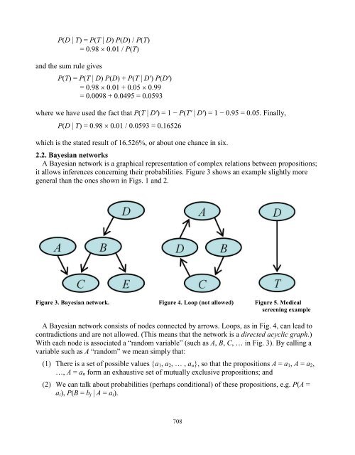
- Page 257: Figure 1. Multiple support for a hy
- Page 261 and 262: For more information about Bayesian
- Page 263 and 264: positive is in the range 0.980 ± 0
- Page 265 and 266: With the notation Emn = “m heads
- Page 267 and 268: 3.1. Selected papers Cravens and Le
- Page 269 and 270: Table 3. P(Eif | Pf) Table 4. P(Ein
- Page 271 and 272: Condensed Matter Nuclear Science”
- Page 273 and 274: 4. J. Breese and D. Koller, “Tuto
- Page 275 and 276: Taking the nuclear origin of copiou
- Page 277 and 278: The evolution of protoscience into
- Page 279 and 280: References 1. Mosier-Boss, P.A., et
- Page 281 and 282: Cold fusion (CF) is a potentially r
- Page 283 and 284: ISCMNS has initiated a CF-dedicated
- Page 285 and 286: Table 2. Current Methods and Propos
- Page 287 and 288: For the CF/OSSc project, the ISCMNS
- Page 289 and 290: ole of skeptical mainstream physici
- Page 291 and 292: sized Pd and Pd alloy particles. Ap
- Page 293 and 294: Honoring Pioneers For most fields o
- Page 295 and 296: A&Z introduced new terms to describ
- Page 297 and 298: The top portion of Fig. 3 shows plo
- Page 299 and 300: Figure 7. New catalyst shows nano-P
- Page 301 and 302: catalyst to outer vessel wall is 7
- Page 303 and 304: Establishment of the “Solid Fusio
- Page 305 and 306: Figure 1. Experimental Device Figur
- Page 307 and 308: [The protocol for producing the ZrO
- Page 309 and 310:
Figure 5A. Comparison of generation
- Page 311 and 312:
Figure 6. Gas pressure characterist
- Page 313 and 314:
Note on Sources The Abstract is a r
- Page 315 and 316:
37. Arata Y, Zhang Y-C; Proc. Japan
- Page 317 and 318:
LENR Research using Co-Deposition S
- Page 319 and 320:
that the tritium production was spo
- Page 321 and 322:
(a) (b) (c) Figure 4. Images obtain
- Page 323 and 324:
SPAWAR Systems Center-Pacific Pd:D
- Page 325 and 326:
7. S. Szpak, P.A. Mosier-Boss, S.R.
- Page 327 and 328:
17. S. Szpak, P.A. Mosier-Boss, and
- Page 329 and 330:
Preparata Prize Acceptance Speech I
- Page 331 and 332:
Cold Fusion Country History Project
- Page 333 and 334:
2. “Condensed Matter Nuclear Scie
- Page 335 and 336:
need for a coordinated effort in ma
- Page 337 and 338:
Colloid J. USSR 48, 8(1986)). In 19
- Page 339 and 340:
scientists on the problem of Cold F
- Page 341 and 342:
Financial support for the conferenc
- Page 343 and 344:
Author Index Pages are in Volume 1
- Page 345:
Wang, J., 299 Watanabe, A., 338 Wei