Williams-Climate-change-refugia-for-terrestrial-biodiversity_0

More documents

Recommendations

Info

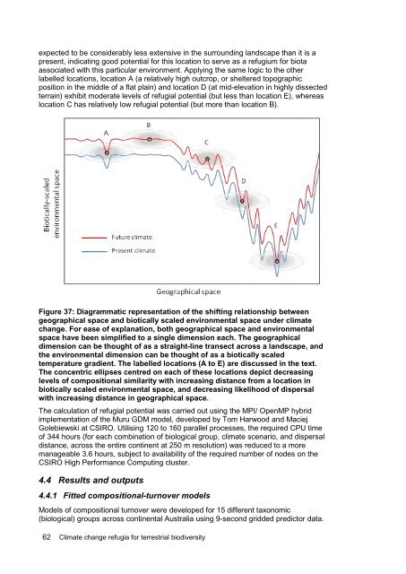
expected to be considerably less extensive in the surrounding landscape than it is a present, indicating good potential for this location to serve as a refugium for biota associated with this particular environment. Applying the same logic to the other labelled locations, location A (a relatively high outcrop, or sheltered topographic position in the middle of a flat plain) and location D (at mid-elevation in highly dissected terrain) exhibit moderate levels of refugial potential (but less than location E), whereas location C has relatively low refugial potential (but more than location B). Figure 37: Diagrammatic representation of the shifting relationship between geographical space and biotically scaled environmental space under climate change. For ease of explanation, both geographical space and environmental space have been simplified to a single dimension each. The geographical dimension can be thought of as a straight-line transect across a landscape, and the environmental dimension can be thought of as a biotically scaled temperature gradient. The labelled locations (A to E) are discussed in the text. The concentric ellipses centred on each of these locations depict decreasing levels of compositional similarity with increasing distance from a location in biotically scaled environmental space, and decreasing likelihood of dispersal with increasing distance in geographical space. The calculation of refugial potential was carried out using the MPI/ OpenMP hybrid implementation of the Muru GDM model, developed by Tom Harwood and Maciej Golebiewski at CSIRO. Utilising 120 to 160 parallel processes, the required CPU time of 344 hours (for each combination of biological group, climate scenario, and dispersal distance, across the entire continent at 250 m resolution) was reduced to a more manageable 3.6 hours, subject to availability of the required number of nodes on the CSIRO High Performance Computing cluster. 4.4 Results and outputs 4.4.1 Fitted compositional-turnover models Models of compositional turnover were developed for 15 different taxonomic (biological) groups across continental Australia using 9-second gridded predictor data. 62 Climate change refugia for terrestrial biodiversity
Models of compositional turnover in vascular plants were also developed using floristic survey data for three regions: all of NSW (3-second resolution), south-east NSW (3second resolution), and the Tingle Mosaic in south-west Western Australia (1-second resolution) (Table 4). Environmental predictors overall explained substantially more of compositional-turnover patterns (estimated from the sum of coefficients fitted to each predictor) than did geographic distance in all models except that for amphibians, where geographic distance was marginally more important (see details in APPENDIX 7. Compositional turnover modelling). As expected, climate variables were the strongest predictors of compositional turnover, particularly among the continental models, compared with regolith (soil and related proxies) and landform variables. Regolith was proportionally more important for most plant groups, especially the nitrogen-fixing Fabales and for the local model of the Tingle Mosaic. All models included one or more of the topographically adjusted climate variables. The continental models incorporated the index of topographic-moisture (EAA) derived from the 9-second MODIS actual evapo-transpiration dataset. This variable was amongst the most important climatic predictors along with continental patterns of summer to winter rainfall seasonality (PTS1), maximum precipitation deficit (WDI) and minimum temperature regimes (TXI, TNX) (see APPENDIX 6. Environmental variables used in GDM modelling for definitions of variables). Table 2: Fitted compositional-turnover (GDM) models. Continental models were applied to the taxonomic subgroups using presence data (first 15 groups listed) and regional models were applied to presence–absence survey data of vascular plants (last three groups listed). Taxonomic group % deviance explained Summed coefficients # predictors Class Mammalia (mammals) 32.40 9.96 20 Class Aves (birds) 24.79 4.60 11 Class Reptilia (reptiles) 37.07 13.30 18 Class Amphibia (amphibians) 45.33 19.50 19 Order Apocrita (wasps and bees) 20.14 16.48 16 Order Coleoptera (beetles) 22.57 13.80 19 Order Aranae (spiders) 20.91 18.40 20 Order Asparagales (lilies and onions) 21.67 17.92 17 Order Asterales (daisies) 37.83 26.51 18 Order Fabales (peas) 37.62 20.12 22 Division Gymnospermae (fruitless seed plants) 35.17 24.47 20 Order Myrtales 29.09 19.59 19 Order Poales (grasses and sedges) 48.17 25.94 19 Order Proteales 42.57 35.06 20 Kingdom Fungi 49.64 34.12 20 NSW plant survey1 45.78 14.00 20 Southeast NSW plant surveys2 33.82 10.59 17 Tingle Mosaic plant surveys1 26.27 6.75 14 1. Vascular plants – ferns and allies, gymnosperms and angiosperms 2. Trees capable of reaching the canopy (includes gymnosperms and some angiosperms) 4.4.2 Refugial potential – Continental 9-second analyses Due to the considerable computation time required to run each of the continental refugial potential analyses (section 4.3.8), the full analytical process was completed for only four of the 15 biological groups: Order Proteales (banksias, grevilleas etc.), Order Fabales (peas, including acacias), reptiles and amphibians. However, all required inputs for the remaining biological groups have been prepared, including all projected environmental variables, biotically scaled at 250 m resolution, using the fitted GDMs for these groups. Potential therefore exists to undertake the final stage of processing; that Climate change refugia for terrestrial biodiversity 63
Page 1:
Climate change refugia for terrestr
Page 4 and 5:
Published by the National Climate C
Page 6 and 7:
3.4.4 Future: current-2085 ........
Page 8 and 9:
APPENDIX 3. Species distribution mo
Page 10 and 11:
Figure 29: A detailed view of the p
Page 12 and 13:
x Climate change refugia for terres
Page 14 and 15:
EXECUTIVE SUMMARY Climate change is
Page 16 and 17:
we will be in a better position to
Page 18 and 19:
1.2.2 Case study 2: Pleistocene sta
Page 20 and 21:
efugia meeting this latter criterio
Page 22 and 23:
2.7 Conclusions Natural systems are
Page 24 and 25: highest RCP reported in the SRES (A
Page 26 and 27: 3.3.4 Species data The study genera
Page 28 and 29: AUC score is negatively correlated
Page 30 and 31: Finally, we assess climate change t
Page 32 and 33: Territory, the Great Australian Big
Page 34 and 35: Figure 5: The 10 th percentile of l
Page 36 and 37: Figure 8: The absolute predicted ch
Page 38 and 39: 3.4.5 Distance measures At a given
Page 40 and 41: the continent, the required movemen
Page 42 and 43: Figure 16: An example of a species
Page 44 and 45: Figure 18: Species richness for eac
Page 46 and 47: Figure 20: The number of immigrants
Page 48 and 49: Figure 22 (cont.): The ‘Immigrant
Page 50 and 51: Figure 24 (cont.): The immigrants a
Page 52 and 53: Figure 26 (cont.): The areas with t
Page 54 and 55: 3.4.7.6 Areas of stability Understa
Page 56 and 57: including the Nullarbor Regional Re
Page 58 and 59: Table 2: The different classes of r
Page 60 and 61: most of the continent by 2085 that
Page 62 and 63: 3.7 Gaps and future research The ne
Page 64 and 65: individual species) will respond to
Page 66 and 67: 4.3.2 Topographically adjusted clim
Page 68 and 69: Tmax adj 0.5° GCM change grids (19
Page 70 and 71: Table 1: Biological groups compiled
Page 72 and 73: Invoking space-for-time substitutio
Page 76 and 77: is, the refugial analysis itself, f
Page 78 and 79: Figure 40: Refugial potential based
Page 80 and 81: Figure 43: Enlarged portion (Kimber
Page 82 and 83: Figure 46: Enlarged portion (Sydney
Page 84 and 85: Figure 48: Inclusion of areas of hi
Page 86 and 87: Figure 51: Refugial potential in th
Page 88 and 89: 4.6 Gaps and future research The GD
Page 90 and 91: 5.3 Research activities and methods
Page 92 and 93: time periods to a distance calculat
Page 94 and 95: proportion of this suitability foun
Page 96 and 97: (a) Figure 54: Stability of the cli
Page 98 and 99: Figure 55: Climate and habitat suit
Page 100 and 101: Mountains in Queensland, the Eungel
Page 102 and 103: Figure 58: Areas of endemism in the
Page 104 and 105: Northern Tablellands Figure 60: Gla
Page 106 and 107: 5.6 Discussion 5.6.1 Endemism in re
Page 108 and 109: (back to 120 kya compared to LGM in
Page 110 and 111: Within each sub-region, potential e
Page 112 and 113: Table 9: Greenspot statistics for o
Page 114 and 115: drought micro-refuges, then targete
Page 116 and 117: The iterative recalculation of all
Page 118 and 119: Figure 64: Zonation conservation pr
Page 120 and 121: 7.6 Gaps and future research The co
Page 122 and 123: Figure 66: The refugia areas result
Page 124 and 125:
8.1.3 Overall lessons from the diff
Page 126 and 127:
9. GAPS AND FUTURE RESEARCH DIRECTI
Page 128 and 129:
REFERENCES Ackerly, D. D., S. R. Lo
Page 130 and 131:
Couper, P. J., B. Hamley, and C. J.
Page 132 and 133:
Winton, A. T. Wittenberg, F. Zeng,
Page 134 and 135:
A. Utteridge, J. E. Watkins, R. Wil
Page 136 and 137:
R Development Core Team. 2011. R: A
Page 138 and 139:
Tingley, M. W., W. B. Monahan, S. R
Page 140 and 141:
APPENDIX 1. CLIMATE SCENARIOS AND B
Page 142 and 143:
Table A1-4: Eighteen Global Climate
Page 144 and 145:
Table A1-5: Thirty-year climate cov
Page 146 and 147:
Figure A2-68. Change in temperature
Page 148 and 149:
Figure A2-70. Proportionate change
Page 150 and 151:
Figure A2-72. The distance an organ
Page 152 and 153:
Figure A2-74. The areas for which t
Page 154 and 155:
APPENDIX 3. SPECIES DISTRIBUTION MO
Page 156 and 157:
APPENDIX 4. PROJECTED SPECIES RICHN
Page 158 and 159:
Figure A4-2. The species richness s
Page 160 and 161:
Table of contents ABSTRACT ........
Page 162 and 163:
INTRODUCTION Terrain modifies local
Page 164 and 165:
RESEARCH ACTIVITIES AND METHODS Dat
Page 166 and 167:
Land Cover The Geosciences Australi
Page 168 and 169:
Figure A5-4: Terrain adjusted model
Page 170 and 171:
RESULTS AND OUTPUTS Figures 8 and 9
Page 172 and 173:
Figure A5-10 Channel Country (SW Qu
Page 174 and 175:
REFERENCES ANU Fenner School of Env
Page 176 and 177:
APPENDIX 6. ENVIRONMENTAL VARIABLES
Page 178 and 179:
Group Short name Name Units Source
Page 180 and 181:
Group Short name Name Units Source
Page 182 and 183:
Data Citations Bureau of Rural Scie
Page 184 and 185:
APPENDIX 7. COMPOSITIONAL TURNOVER
Page 186 and 187:
Table A7-9. Vascular plant data app
Page 188 and 189:
to support in house applications an
Page 190 and 191:
Table A7-10. Summary of GDM model f
Page 192 and 193:
Variable Group Predictor variable a
Page 194 and 195:
a) c) Figure A7-78. Continental Aus
Page 196 and 197:
Page 198 and 199:
Page 200 and 201:
Page 202 and 203:
Page 204 and 205:
Page 206 and 207:
Page 208 and 209:
Table A7-15. Overall relative impor
Page 210 and 211:
a) c) Figure A7-92. Eastern Austral
Page 212 and 213:
Table A7-18. Overall relative impor
Page 214 and 215:
a) c) Figure A7-94. Tingle Mosaic s
Page 216 and 217:
References Allen R, Pereira L, Raes
Page 218 and 219:
APPENDIX 8. PLEISTOCENE STABILITY A
Page 220 and 221:
Figure A8-3. Rainforest in the Aust
Page 222 and 223:
Canis lupus dingo CANLUPU MAMM Cani
Page 224 and 225:
Lampropholis mirabilis LAMMIRA REPT
Page 226 and 227:
Stegonotus cucullatus STECUCU REPT
Page 228:
Figure A10-1. Spatial patterns of v
show all

Williams-Climate-change-refugia-for-terrestrial-biodiversity_0

You also want an ePaper? Increase the reach of your titles

Delete template?

Save as template?