Boundary Lyer Theory

192
JX. 1Cxact sol~tLion~ of tho stmdy-state l~ountlary-layer equat,iona i. Tho method of finite diffcfcrrnoes 103
R, and G',, for sucoessive values of n startling wit,h ?z = 2 for all grid point,s between
the wall and the edge of the 1)onndary layer.
Sinco 17,,.,l for 12 = N-1 is known from rqnat,ion (!).70), it lmx~mcs possible to
evaluate all nnlznowns F, by means of equation (9.77) whilc t,mversing td~o boundary
layer from t,ho edge t,o t,he wall tJlrongll (Icrreasing va111cs of n, i. c. for 17. -- N-l ,
N--2, . . ., 2. '1'11is cornplr1,rs lhr cdc1lln1,ion of Il',, (7.- F,, ll.n) in ono it.c~.nl,ion. On(:(:
I{',,,, 1111s I)c~w tlr~r~~nii~~r(l. thr cot.~.c.sj)ondi~ig solntion for /0141,n ca.n be found by
rlireot. nun~wirnl inhcgrxt,ion of equat'ion (9.05). The t,rapezoidal rule snfficcs for t,his
purpose.
The calculat.et1 vniues P7n4.1,n a.nd /,,+l,. are used t,o dntmnline new and improved
,.
valrtcs of t,he coc,fficients A,,, I?,,, C,, which in t,urn leads t,o new and improved values
of F,+I,,, antl f,, , I,,. 111~ ~WOCCSS is t.~rmin:~tcd when t,hc rcsnlt,~ of two s~~cccssivc
it,rrnt,ions ngrco t,o within a specified tdcrancc, typically of order 10-5. 'l'ho convergrnce
is nsnallp rapid, t01ree t,o four iterations being adequate in most cases with
st,rp sizrs A.r in l,he range 0.01 t,o 0.05.
In crrt,t~in pro11lc:nis it, I~ecomrs n~ccssnr~ t,o nllow for bonnda.ry-li~y(~ growt,l~
1)y inrrc,asing N (or ve) as t,hr calcnlatrions proceed tlownst,reant. The houndarylayer
edge is rlcfinctl by thr rcquircmcnt t,hat tho difference FN-Fnr~l should be
Iws t,lian a sprrificd value, t,.vpically of ordrr 10-4. 7'hc growth, in t,crrns of the presrnt
variablcs, is usually very modest even for cases involving separation.
A vnrial~lc of primary intcrcst. in the calcnlat,ion is the s1.rrs.s at t,hc wall; it,s
vnluo can bc tl~t~erminetl with good accuracy from the five point formula
Iuirinl vnlr~cs: \Vlic~n using hnl111lrr1.c.tl similar solrrl.ions as s1,arling vdrlcs, ext,c:nsivc
int~c~t,j)olat,ioti is rcclnirecl whrncver variable step sizes Ay,, are nsctl. It is
rnorcx convcnirnt, antl efficient also t,tr gcnerate t,hc sin~ilarit~y solut.ion by finite
tlifi~rr-rcs t.hroupl1 surcrssivc iterat,ions. The equat,ion t>o be solved is oht,aincd from
cclna,li~m (!).64). and can I)c writtam in 1inoar.ized form as
guessing a so la ti or^ which salisfics the boundary condit,ions), whereas those wit,ll
index i arc to be found in the 1:-th or cnrrcnt itcmt,ion. 'L'lte tlifTcrc:nc:c quol,irnf,s
(9.69) and (0.70) are now snl)stitut,cd ink) equa0ion (!).84). 'I'hc rrsult. is a tlilli~~~~ncc
equat,ion which can be writt,en in the standard form of eqnat,ion (9.74), with coeffi -
A linear variation in F suffices as an initid guess, Fo, and the corrcspontling value
off is detmmincd from equation (9.86). The coefficients A,, /I,,, C,, and I),, nro (XIoulntcd
next, and tltc corresponcling vnlncs of /?,, and (r,, arc tlct~errninctl ~~eross thtbonntlary
layer. The recurrence rclnlion (9.77) and t,he bountlnrg contlit,iorls (!).78)
are then used to determine the new it,crat.e, FI, across thr bounclnry lager. 'Yhr
process is repeated until the difference bct,wcen successive it,eratrs becomes smaller
than the specified t,olerance. The number of it.emtions required is typically of order
8 to 12. The method is simpler t,llan t,he usl~al W~ooting'' ~ncthod used for two-point
lmnntlary-vnlnc problem$ arid it converges in many rases WIICIT t,lrc In,t.ter mct,l~otl
fails, for inst,ance for very large blowing mt.cs.
Applications: The finite-difference method prescnt.ctl hrrc is in1,cntlctl as n prnctical
engineering t,ool. Great,rr accuracy cnn be achicvcrl with a more clalwrntr procedure,
1,111, t,his in turn leads t,o greater cotnplexit,y in fornlnlat,ion mtl progrnmrning
and to an increased demnlid for computm t,ime and cnpacit.y. The conipnting time
nnd accnmey tlrpcnd for all tlifTcrcncc ntet,lrotls on the skp sizr nsrtl in thr rnlrw
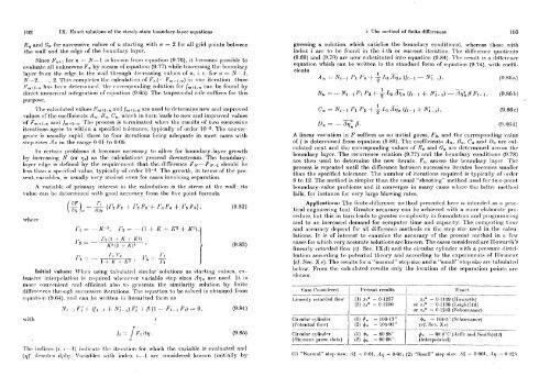
Iations. It, is of int.crest, to exa,mine the accuracy of the present, mct,hotl in a few
cases for which very accurat3e solut,ions are known. The cases considrretl are 11owa1~t.h'~
linrnrly retarded flow (cf. Scc. IXd) a,nd the circular cylinder with a pressure clistrihut.ion
ncrortling 1,o pot.cnt,inl 1.hrory and nccotding t,o t.hc cspcriments of I[ic.n~r~lz
(c/. See. X c). '1'11~ rrsult,s for n "normnl" step sizc and a "srnnll" step size arc tabnlntcd
11clow. lhtn t.11~ C:IICIII:L~~ rcs1111~s only the locat.ion of the scl~n.rt~.l.ion 11oin1s IIII!
sl~own.
Case ('o~kIerrd 1 Present redts 1Sxnct
1,inenrly set.artlrtl Ilow
Circular ryli~~tlcr
(l'okntinl flow)
-.
Circular cylit)tlrr
(Ilic~ncne prms. tlntn)
I
(1) x,' = 0.1227
(2) x,* = 0.1210
(1) 4, = 106.13"
(2) 4, = 105.01 O
r8* = 0.1 I!)!) (Ilownrtli)
or r,* = 0.1 198 (l,eig11)[44]
I or T,* - 0.1203 (Sc4~ortinr~~)
4a - 104.5' (Srl~ocnni~er)
(rf. Scc. Xc)
--
(I) $, = 80.98"
(2) 4, = 80.08"
#. -= 80WC (.lnlli: nnd Stnitl1)(.42/
(interl)olntrd)
.-