Study Guide and Intervention (continued) - MathnMind
Study Guide and Intervention (continued) - MathnMind
Study Guide and Intervention (continued) - MathnMind

Create successful ePaper yourself
Turn your PDF publications into a flip-book with our unique Google optimized e-Paper software.
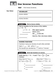
14-4<br />
Probability Distributions The probabilities associated with every possible value of<br />
the r<strong>and</strong>om variable X make up what are called the probability distribution for that<br />
variable. A probability distribution has the following properties.<br />
Properties of a 1. The probability of each value of X is greater than or equal to 0.<br />
Probability Distribution 2. The probabilities for all values of X add up to 1.<br />
The probability distribution for a r<strong>and</strong>om variable can be given in a table or in a<br />
probability histogram <strong>and</strong> used to obtain other information.<br />
Example<br />
NAME ______________________________________________ DATE______________ PERIOD _____<br />
<strong>Study</strong> <strong>Guide</strong> <strong>and</strong> <strong>Intervention</strong> (<strong>continued</strong>)<br />
Probability Distributions<br />
The data from the example on page 849 can be used to determine a<br />
probability distribution <strong>and</strong> to make a probability histogram.<br />
X Number of Siblings P (X )<br />
a. Show that the probability<br />
distribution is valid.<br />
Exercises<br />
0 0.037<br />
1 0.556<br />
2 0.296<br />
3 0.074<br />
4 0.037<br />
For each value of X, the probability<br />
is greater than or equal to 0 <strong>and</strong><br />
less than or equal to 1. Also, the<br />
sum of the probabilities is 1.<br />
© Glencoe/McGraw-Hill 850 Glencoe Algebra 1<br />
0.600<br />
0.400<br />
P(X)<br />
0.200<br />
The table at the right shows the probability<br />
distribution for students by school enrollment in the<br />
United States in 1997. Use the table for Exercises 1–3.<br />
1. Show that the probability distribution is valid.<br />
2. If a student is chosen at r<strong>and</strong>om, what is the probability<br />
that the student is in elementary or secondary school?<br />
3. Make a probability histogram of the data.<br />
Probability Histogram<br />
0 1 2 3 4<br />
X Number of Siblings<br />
b. What is the probability that a student<br />
chosen at r<strong>and</strong>om has fewer than<br />
2 siblings?<br />
Because the events are independent, the<br />
probability of fewer than 2 siblings is the sum of<br />
the probability of 0 siblings <strong>and</strong> the probability<br />
of 1 sibling, or 0.037 0.556 0.593.<br />
X Type of School P (X )<br />
Elementary 1 0.562<br />
Secondary 2 0.219<br />
Higher Education 3 0.219<br />
Source: The New York Times Almanac<br />
1.0<br />
0.8<br />
P(X) 0.6<br />
0.4<br />
0.2<br />
Probability Histogram<br />
1 2 3<br />
X Type of School