Itinerant Spin Dynamics in Structures of ... - Jacobs University

Chapter 3: WL/WAL Crossover and Spin Relaxation in Confined Systems 29
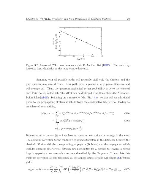
Figure 3.2: Measured WL corrections on a thin PdAu film, Ref.[DO79]. The resistivity
increases logarithmically as the temperature decreases.
Summing over all possible paths will generally yield only the classical and the
pure quantum-mechanical term. Other path have in general a large phase difference and
will average out. Thus, the quantum-mechanical return-probability is twice the classical
one. This effect is called WL. This effect can be destroyed if we think about the Aharonov-
Bohm-Effect[AB59]: Switching on a magnetic field, Fig.(3.3), we can add an additional
phase to the propagating electron which destroys the constructive interference, leading to
an enhanced conductivity,
|P(r,r)| 2 ≈ ∑ α
= ∑ α
〈(A αe i2πϕ +A αe −i2πϕ )(A ∗
α e −i2πϕ +A ∗
α e i2πϕ )〉 (3.5)
〈2|A α| 2 (1+cos(4πϕ))〉 (3.6)
with ϕ = φ/φ 0 ,φ 0 = h e .
Because of 〈(1 +cos(4πϕ))〉 = 1 we have no quantum corrections on average in this case.
The quantum correction to the conductivity appears therefore in the difference between the
classical diffusion with the corresponding propagator (Diffuson) and the propagation which
includes quantum interference between two possibilities for a particle to traverse a closed
loop in opposite -time reversed- directions described by the Cooperon. To calculate this
quantum correction at zero frequency ω, one applies Kubo formula (Appendix B.1) which
yields
σ xx (ω = 0) ≡ σ = e2 2π
m 2 e Vol
∫ ∞
0
dE
(
− ∂f(E) )
〈Tr[δ(E −H 0 )p x δ(E −H 0 )p x ]〉
∂E
imp
. (3.7)