Itinerant Spin Dynamics in Structures of ... - Jacobs University

36 Chapter 3: WL/WAL Crossover and Spin Relaxation in Confined Systems
It follows that for weak disorder and without Zeeman coupling, the Cooperon depends only
on the total momentum Q and the total spin S. Expanding the Cooperon to second order
in (Q+2eA+2m e âS) and performing the angular integral which is for 2D diffusion (elastic
mean-free path l e smaller than wire width W) continuous from 0 to 2π and yields
Ĉ(Q) =
1
D e (Q+2eA+2eA S ) 2 +H γD
. (3.43)
The effective vector potential due to SO interaction, A S = m eˆαS/e (where ˆα = 〈â〉 denotes
the matrix Eq.(3.40), as averaged over angle), couples to total spin vector S whose components
are four by four matrices. The cubic Dresselhaus coupling is found to reduce the
effect of the linear one to
˜α 1 := α 1 −m e γ D E F /2. (3.44)
Furthermore, it gives rise to the spin relaxation term in Eq.(3.43),
H γD = D e (m 2 e E Fγ D ) 2 (Sx 2 +S2 y ). (3.45)
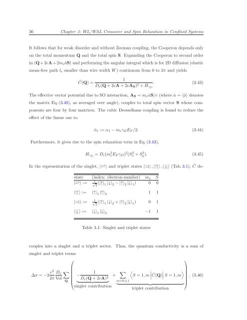
In the representation of the singlet, |⇄〉 and triplet states |⇉〉,|⇈〉,|〉 (Tab.3.1), Ĉ destate
(index: electron-number) m s S
|⇄〉 := 1 √
2
(|↑〉 1
|↓〉 2
−|↑〉 2
|↓〉 1
) 0 0
|⇈〉 := |↑〉 1
|↑〉 2
1 1
|⇉〉 := 1 √
2
(|↑〉 1
|↓〉 2
+|↑〉 2
|↓〉 1
) 0 1
|〉 := |↓〉 1
|↓〉 2
−1 1
Table 3.1: Singlet and triplet states
couples into a singlet and a triplet sector. Thus, the quantum conductivity is a sum of
singlet and triplet terms
⎛
∆σ = −2 e2 D e
2π Vol
∑
1
−
⎜ D
Q ⎝ e (Q+2eA)
} {{ 2 + ∑
}
singlet contribution
〈
∣ 〉
∣ ∣∣S
S = 1,m ∣Ĉ(Q) = 1,m . (3.46)
⎟
m=0,±1
⎠
} {{ }
triplet contribution
⎞