Michael Corral: Vector Calculus

1.1 Introduction 3
You have already dealt with velocity and acceleration in single-variable calculus.
For example, for motion along a straight line, if y= f(t) gives the displacement of
an object after time t, then dy/dt= f ′ (t) is the velocity of the object at time t. The
derivative f ′ (t) is just a number, which is positive if the object is moving in an agreedupon
“positive” direction, and negative if it moves in the opposite of that direction. So
you can think of that number, which was called the velocity of the object, as having
two components: a magnitude, indicated by a nonnegative number, preceded by a
direction, indicated by a plus or minus symbol (representing motion in the positive
direction or the negative direction, respectively), i.e. f ′ (t)=±a for some number a≥0.
Then a is the magnitude of the velocity (normally called the speed of the object), and
the±represents the direction of the velocity (though the+is usually omitted for the
positive direction).
For motion along a straight line, i.e. in a 1-dimensional space, the velocities are
also contained in that 1-dimensional space, since they are just numbers. For general
motion along a curve in 2- or 3-dimensional space, however, velocity will need to be
represented by a multidimensional object which should have both a magnitude and a
direction. A geometric object which has those features is an arrow, which in elementary
geometry is called a “directed line segment”. This is the motivation for how we
will define a vector.
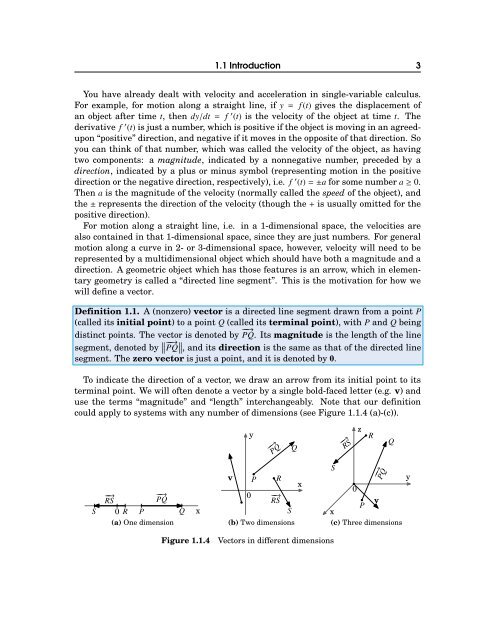
Definition 1.1. A (nonzero) vector is a directed line segment drawn from a point P
(called its initial point) to a point Q (called its terminal point), with P and Q being
distinct points. The vector is denoted by −→ PQ. Its magnitude is the length of the line
segment, denoted by ∥ −→∥ ∥PQ ∥∥, and its direction is the same as that of the directed line
segment. The zero vector is just a point, and it is denoted by 0.
To indicate the direction of a vector, we draw an arrow from its initial point to its
terminal point. We will often denote a vector by a single bold-faced letter (e.g. v) and
use the terms “magnitude” and “length” interchangeably. Note that our definition
could apply to systems with any number of dimensions (see Figure 1.1.4 (a)-(c)).
y
−→ PQ
Q
−→ RS
z
R
Q
S
−→ −→
RS PQ
0 R P Q x
(a) One dimension
v
0
P
R
−→
RS
S
(b) Two dimensions
x
S
x
0
P
−→ PQ
v
(c) Three dimensions
y
Figure 1.1.4 Vectors in different dimensions