Michael Corral: Vector Calculus

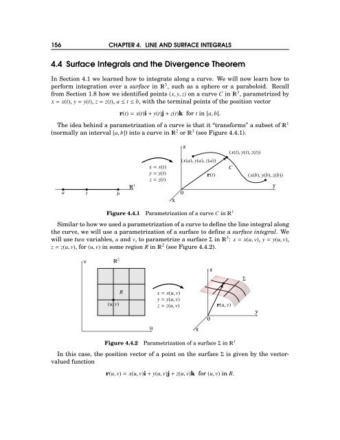
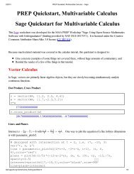
156 CHAPTER 4. LINE AND SURFACE INTEGRALS
4.4 Surface Integrals and the Divergence Theorem
In Section 4.1 we learned how to integrate along a curve. We will now learn how to
perform integration over a surface in 3 , such as a sphere or a paraboloid. Recall
from Section 1.8 how we identified points (x,y,z) on a curve C in 3 , parametrized by
x= x(t), y=y(t), z=z(t), a≤t≤b, with the terminal points of the position vector
r(t)= x(t)i+y(t)j+z(t)k for t in [a,b].
The idea behind a parametrization of a curve is that it “transforms” a subset of 1
(normally an interval [a,b]) into a curve in 2 or 3 (see Figure 4.4.1).
a t b
1
x= x(t)
y=y(t)
z=z(t)
x
z
(x(a),y(a),z(a))
r(t)
0
(x(t),y(t),z(t))
C
(x(b),y(b),z(b))
y
Figure 4.4.1 Parametrization of a curve C in 3
Similartohowweusedaparametrizationofacurvetodefinethelineintegralalong
the curve, we will use a parametrization of a surface to define a surface integral. We
will use two variables, u and v, to parametrize a surfaceΣin 3 : x= x(u,v), y=y(u,v),
z=z(u,v), for (u,v) in some region R in 2 (see Figure 4.4.2).
v
2
z
Σ
(u,v)
R
x= x(u,v)
y=y(u,v)
z=z(u,v)
0
r(u,v)
y
u
x
Figure 4.4.2 Parametrization of a surfaceΣin 3
In this case, the position vector of a point on the surfaceΣis given by the vectorvalued
function
r(u,v)= x(u,v)i+y(u,v)j+z(u,v)k for (u,v) in R.