Michael Corral: Vector Calculus
Michael Corral: Vector Calculus
Michael Corral: Vector Calculus

Create successful ePaper yourself
Turn your PDF publications into a flip-book with our unique Google optimized e-Paper software.
1.8 <strong>Vector</strong>-Valued Functions 51<br />
1.8 <strong>Vector</strong>-Valued Functions<br />
Now that we are familiar with vectors and their operations, we can begin discussing<br />
functions whose values are vectors.<br />
Definition 1.10. A vector-valued function of a real variable is a rule that associates<br />
a vector f(t) with a real number t, where t is in some subset D of 1 (called the<br />
domain of f). We write f : D→ 3 to denote that f is a mapping of D into 3 .<br />
For example, f(t)=ti+t 2 j+t 3 k is a vector-valued function in 3 , defined for all real<br />
numbers t. We would write f :→ 3 . At t=1the value of the function is the vector<br />
i+j+k, which in Cartesian coordinates has the terminal point (1,1,1).<br />
A vector-valued function of a real variable can be written in component form as<br />
or in the form<br />
f(t)= f 1 (t)i+ f 2 (t)j+ f 3 (t)k<br />
f(t)=(f 1 (t), f 2 (t), f 3 (t))<br />
for some real-valued functions f 1 (t), f 2 (t), f 3 (t), called the component functions of f. The<br />
first form is often used when emphasizing that f(t) is a vector, and the second form is<br />
usefulwhenconsideringjusttheterminalpointsofthevectors. Byidentifyingvectors<br />
withtheirterminalpoints,acurveinspacecanbewrittenasavector-valuedfunction.<br />
Example 1.35. Define f :→ 3 by f(t)=(cost,sint,t).<br />
This is the equation of a helix (see Figure 1.8.1). As the value<br />
of t increases, the terminal points of f(t) trace out a curve spiraling<br />
upward. For each t, the x- and y-coordinates of f(t) are<br />
x=cost and y=sint, so<br />
x 2 +y 2 = cos 2 t+sin 2 t=1.<br />
Thus, the curve lies on the surface of the right circular cylinder<br />
x 2 +y 2 = 1.<br />
f(2π)<br />
f(0)<br />
x<br />
0<br />
z<br />
Figure 1.8.1<br />
It may help to think of vector-valued functions of a real variable in 3 as a generalization<br />
of the parametric functions in 2 which you learned about in single-variable<br />
calculus. Much of the theory of real-valued functions of a single real variable can be<br />
applied to vector-valued functions of a real variable. Since each of the three component<br />
functions are real-valued, it will sometimes be the case that results from singlevariable<br />
calculus can simply be applied to each of the component functions to yield<br />
a similar result for the vector-valued function. However, there are times when such<br />
generalizations do not hold (see Exercise 13). The concept of a limit, though, can be<br />
extended naturally to vector-valued functions, as in the following definition.<br />
y