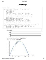
88 CHAPTER 2. FUNCTIONS OF SEVERAL VARIABLES 0.4 0.35 0.3 0.25 0.2 0.15 z 0.1 0.05 0 -3 -2 -1 y 0 1 2 3 3 2 1 0 -1 -2 x -3 Figure 2.5.2 f(x,y)=(x 2 +y 2 )e −(x2 +y 2 ) ☛ ✟ ✡Exercises ✠ A For Exercises 1-10, find all local maxima and minima of the function f(x,y). 1. f(x,y)= x 3 −3x+y 2 2. f(x,y)= x 3 −12x+y 2 +8y 3. f(x,y)= x 3 −3x+y 3 −3y 4. f(x,y)= x 3 +3x 2 +y 3 −3y 2 5. f(x,y)=2x 3 +6xy+3y 2 6. f(x,y)=2x 3 −6xy+y 2 7. f(x,y)= √ x 2 +y 2 8. f(x,y)= x+2y 9. f(x,y)=4x 2 −4xy+2y 2 +10x−6y 10. f(x,y)=−4x 2 +4xy−2y 2 +16x−12y B 11. Forarectangularsolidofvolume1000cubicmeters, findthedimensionsthatwill minimize the surface area. (Hint: Use the volume condition to write the surface area as a function of just two variables.) 12. Prove that if (a,b) is a local maximum or local minimum point for a smooth function f(x,y), then the tangent plane to the surface z= f(x,y) at the point (a,b, f(a,b)) is parallel to the xy-plane. (Hint: Use Theorem 2.5.) C 13. Findthreepositivenumbers x, y, zwhosesumis10suchthat x 2 y 2 zisamaximum.
2.6 Unconstrained Optimization: Numerical Methods 89 2.6 Unconstrained Optimization: Numerical Methods The types of problems that we solved in the previous section were examples of unconstrained optimization problems. That is, we tried to find local (and perhaps even global) maximum and minimum points of real-valued functions f(x,y), where the points (x,y) could be any points in the domain of f. The method we used required us to find the critical points of f, which meant having to solve the equation∇f = 0, which in general is a system of two equations in two unknowns (x and y). While this was relatively simple for the examples we did, in general this will not be the case. If the equations involve polynomials in x and y of degree three or higher, or complicated expressions involving trigonometric, exponential, or logarithmic functions, then solving even one such equation, let alone two, could be impossible by elementary means. 7 For example, if one of the equations that had to be solved was x 3 +9x−2=0, you may have a hard time getting the exact solutions. Trial and error would not help much,especiallysincetheonlyrealsolution 8 turnsouttobe 3√ √ 28+1− 3 √ √ 28−1. Ina situation such as this, the only choice may be to find a solution using some numerical method which gives a sequence of numbers which converge to the actual solution. For example, Newton’s method for solving equations f(x)=0, which you probably learned in single-variable calculus. In this section we will describe another method of Newton for finding critical points of real-valued functions of two variables. Let f(x,y) be a smooth real-valued function, and define D(x,y)= ∂2 f ∂x 2(x,y)∂2 f ∂y 2(x,y)− ( ∂ 2 f ∂y∂x (x,y) ) 2. Newton’s algorithm: Pick an initial point (x 0 ,y 0 ). For n=0,1,2,3,..., define: ∂ 2 f ∂ (x ∂y 2 n ,y n ) 2 f ∂x∂y (x n,y n ) ∂ 2 f ∂ (x ∂f ∣∂y x n+1 = x n − (x ∂f n,y n ) ∂x (x ∂x n,y n ) 2 n ,y n ) 2 f ∂x∂y (x n,y n ) ∣ ∂f ∣∂x , y n+1 = y n − (x ∂f n,y n ) ∂y (x n,y n ) ∣ D(x n ,y n ) D(x n ,y n ) (2.14) Then the sequence of points (x n ,y n ) ∞ n=1 converges to a critical point. If there are several critical points, then you will have to try different initial points to find them. 7 This is also a problem for the equivalent method (the Second Derivative Test) in single-variable calculus, though one that is not usually emphasized. 8 There are also two nonreal, complex number solutions. Cubic polynomial equations in one variable can be solved using Cardan’s formulas, which are not quite as simple as the familiar quadratic formula. See USPENSKY for more details. There are formulas for solving polynomial equations of degree 4, but it can be proved that there is no general formula for solving equations for polynomials of degree five or higher.