- Page 1:
LibraryPirate
- Page 6:
PUBLISHER ACQUISITIONS EDITOR ASSOC
- Page 10:
This page intentionally left blank
- Page 14:
vi PREFACE Chapter 1 Introduction t
- Page 18:
viii PREFACE Edward Danial David El
- Page 22:
x CONTENTS 6.3 The t Distribution 1
- Page 26:
This page intentionally left blank
- Page 30:
2 CHAPTER 1 INTRODUCTION TO BIOSTAT
- Page 34:
4 CHAPTER 1 INTRODUCTION TO BIOSTAT
- Page 38:
6 CHAPTER 1 INTRODUCTION TO BIOSTAT
- Page 42:
8 CHAPTER 1 INTRODUCTION TO BIOSTAT
- Page 46:
10 CHAPTER 1 INTRODUCTION TO BIOSTA
- Page 50:
12 CHAPTER 1 INTRODUCTION TO BIOSTA
- Page 54:
14 CHAPTER 1 INTRODUCTION TO BIOSTA
- Page 58:
16 CHAPTER 1 INTRODUCTION TO BIOSTA
- Page 62:
18 CHAPTER 1 INTRODUCTION TO BIOSTA
- Page 66:
20 CHAPTER 2 DESCRIPTIVE STATISTICS
- Page 70:
22 CHAPTER 2 DESCRIPTIVE STATISTICS
- Page 74:
24 CHAPTER 2 DESCRIPTIVE STATISTICS
- Page 78:
26 CHAPTER 2 DESCRIPTIVE STATISTICS
- Page 82:
28 CHAPTER 2 DESCRIPTIVE STATISTICS
- Page 86:
30 CHAPTER 2 DESCRIPTIVE STATISTICS
- Page 90:
32 CHAPTER 2 DESCRIPTIVE STATISTICS
- Page 94:
34 CHAPTER 2 DESCRIPTIVE STATISTICS
- Page 98:
36 CHAPTER 2 DESCRIPTIVE STATISTICS
- Page 102:
38 CHAPTER 2 DESCRIPTIVE STATISTICS
- Page 106:
40 CHAPTER 2 DESCRIPTIVE STATISTICS
- Page 110:
42 CHAPTER 2 DESCRIPTIVE STATISTICS
- Page 114:
44 CHAPTER 2 DESCRIPTIVE STATISTICS
- Page 118:
46 CHAPTER 2 DESCRIPTIVE STATISTICS
- Page 122:
48 CHAPTER 2 DESCRIPTIVE STATISTICS
- Page 126:
50 CHAPTER 2 DESCRIPTIVE STATISTICS
- Page 130:
52 CHAPTER 2 DESCRIPTIVE STATISTICS
- Page 134:
54 CHAPTER 2 DESCRIPTIVE STATISTICS
- Page 138:
56 CHAPTER 2 DESCRIPTIVE STATISTICS
- Page 142:
58 CHAPTER 2 DESCRIPTIVE STATISTICS
- Page 146:
60 CHAPTER 2 DESCRIPTIVE STATISTICS
- Page 150:
62 CHAPTER 2 DESCRIPTIVE STATISTICS
- Page 154:
64 CHAPTER 2 DESCRIPTIVE STATISTICS
- Page 158:
66 CHAPTER 3 SOME BASIC PROBABILITY
- Page 162:
68 CHAPTER 3 SOME BASIC PROBABILITY
- Page 166:
70 CHAPTER 3 SOME BASIC PROBABILITY
- Page 170:
72 CHAPTER 3 SOME BASIC PROBABILITY
- Page 174:
74 CHAPTER 3 SOME BASIC PROBABILITY
- Page 178:
76 CHAPTER 3 SOME BASIC PROBABILITY
- Page 182:
78 CHAPTER 3 SOME BASIC PROBABILITY
- Page 186:
80 CHAPTER 3 SOME BASIC PROBABILITY
- Page 190:
82 CHAPTER 3 SOME BASIC PROBABILITY
- Page 194:
84 CHAPTER 3 SOME BASIC PROBABILITY
- Page 198:
86 CHAPTER 3 SOME BASIC PROBABILITY
- Page 202:
88 CHAPTER 3 SOME BASIC PROBABILITY
- Page 206:
90 CHAPTER 3 SOME BASIC PROBABILITY
- Page 210:
92 CHAPTER 3 SOME BASIC PROBABILITY
- Page 214:
94 CHAPTER 4 PROBABILITY DISTRIBUTI
- Page 218:
96 CHAPTER 4 PROBABILITY DISTRIBUTI
- Page 222:
98 CHAPTER 4 PROBABILITY DISTRIBUTI
- Page 226:
100 CHAPTER 4 PROBABILITY DISTRIBUT
- Page 230:
102 CHAPTER 4 PROBABILITY DISTRIBUT
- Page 234:
104 CHAPTER 4 PROBABILITY DISTRIBUT
- Page 238:
106 CHAPTER 4 PROBABILITY DISTRIBUT
- Page 242:
108 CHAPTER 4 PROBABILITY DISTRIBUT
- Page 246:
110 CHAPTER 4 PROBABILITY DISTRIBUT
- Page 250:
112 CHAPTER 4 PROBABILITY DISTRIBUT
- Page 254:
114 CHAPTER 4 PROBABILITY DISTRIBUT
- Page 258:
116 CHAPTER 4 PROBABILITY DISTRIBUT
- Page 262:
118 CHAPTER 4 PROBABILITY DISTRIBUT
- Page 266:
120 CHAPTER 4 PROBABILITY DISTRIBUT
- Page 270:
122 CHAPTER 4 PROBABILITY DISTRIBUT
- Page 274:
124 CHAPTER 4 PROBABILITY DISTRIBUT
- Page 278:
126 CHAPTER 4 PROBABILITY DISTRIBUT
- Page 282:
128 CHAPTER 4 PROBABILITY DISTRIBUT
- Page 286:
130 CHAPTER 4 PROBABILITY DISTRIBUT
- Page 290:
132 CHAPTER 4 PROBABILITY DISTRIBUT
- Page 294:
134 CHAPTER 4 PROBABILITY DISTRIBUT
- Page 298:
136 CHAPTER 5 SOME IMPORTANT SAMPLI
- Page 302:
138 CHAPTER 5 SOME IMPORTANT SAMPLI
- Page 306:
140 CHAPTER 5 SOME IMPORTANT SAMPLI
- Page 310:
142 CHAPTER 5 SOME IMPORTANT SAMPLI
- Page 314:
144 CHAPTER 5 SOME IMPORTANT SAMPLI
- Page 318:
146 CHAPTER 5 SOME IMPORTANT SAMPLI
- Page 322:
148 CHAPTER 5 SOME IMPORTANT SAMPLI
- Page 326:
150 CHAPTER 5 SOME IMPORTANT SAMPLI
- Page 330:
152 CHAPTER 5 SOME IMPORTANT SAMPLI
- Page 334:
154 CHAPTER 5 SOME IMPORTANT SAMPLI
- Page 338:
156 CHAPTER 5 SOME IMPORTANT SAMPLI
- Page 342:
158 CHAPTER 5 SOME IMPORTANT SAMPLI
- Page 346:
160 CHAPTER 5 SOME IMPORTANT SAMPLI
- Page 350:
CHAPTER6 ESTIMATION CHAPTER OVERVIE
- Page 354:
164 CHAPTER 6 ESTIMATION We will fi
- Page 358:
166 CHAPTER 6 ESTIMATION many insta
- Page 362:
168 CHAPTER 6 ESTIMATION Interval E
- Page 366:
170 CHAPTER 6 ESTIMATION Solution:
- Page 370:
172 CHAPTER 6 ESTIMATION someone wh
- Page 374:
174 CHAPTER 6 ESTIMATION Normal dis
- Page 378:
176 CHAPTER 6 ESTIMATION Yes Popula
- Page 382:
178 CHAPTER 6 ESTIMATION Construct
- Page 386:
180 CHAPTER 6 ESTIMATION By Equatio
- Page 390:
182 CHAPTER 6 ESTIMATION The proble
- Page 394:
184 CHAPTER 6 ESTIMATION error of t
- Page 398:
186 CHAPTER 6 ESTIMATION distributi
- Page 402:
188 CHAPTER 6 ESTIMATION EXAMPLE 6.
- Page 406:
190 CHAPTER 6 ESTIMATION since the
- Page 410:
192 CHAPTER 6 ESTIMATION age of per
- Page 414:
194 CHAPTER 6 ESTIMATION 6.9 CONFID
- Page 418:
196 CHAPTER 6 ESTIMATION FIGURE 6.9
- Page 422:
198 CHAPTER 6 ESTIMATION for s 2 ,
- Page 426:
200 CHAPTER 6 ESTIMATION f (x) 1.0
- Page 430:
202 CHAPTER 6 ESTIMATION the column
- Page 434:
204 CHAPTER 6 ESTIMATION SUMMARY OF
- Page 438:
206 CHAPTER 6 ESTIMATION • df de
- Page 442:
208 CHAPTER 6 ESTIMATION 22. Determ
- Page 446:
210 CHAPTER 6 ESTIMATION 29. The pu
- Page 450:
212 CHAPTER 6 ESTIMATION 7. Refer t
- Page 454:
214 CHAPTER 6 ESTIMATION A-26. MOHE
- Page 458:
216 CHAPTER 7 HYPOTHESIS TESTING 7.
- Page 462:
218 CHAPTER 7 HYPOTHESIS TESTING Ru
- Page 466:
220 CHAPTER 7 HYPOTHESIS TESTING st
- Page 470:
222 CHAPTER 7 HYPOTHESIS TESTING Ev
- Page 474:
224 CHAPTER 7 HYPOTHESIS TESTING th
- Page 478:
226 CHAPTER 7 HYPOTHESIS TESTING ca
- Page 482:
228 CHAPTER 7 HYPOTHESIS TESTING at
- Page 486:
230 CHAPTER 7 HYPOTHESIS TESTING So
- Page 490:
232 CHAPTER 7 HYPOTHESIS TESTING is
- Page 494:
234 CHAPTER 7 HYPOTHESIS TESTING Di
- Page 498:
236 CHAPTER 7 HYPOTHESIS TESTING 7.
- Page 502:
238 CHAPTER 7 HYPOTHESIS TESTING wh
- Page 506:
240 CHAPTER 7 HYPOTHESIS TESTING EX
- Page 510:
242 CHAPTER 7 HYPOTHESIS TESTING to
- Page 514:
244 CHAPTER 7 HYPOTHESIS TESTING We
- Page 518:
246 CHAPTER 7 HYPOTHESIS TESTING Th
- Page 522:
248 CHAPTER 7 HYPOTHESIS TESTING To
- Page 526:
250 CHAPTER 7 HYPOTHESIS TESTING 7.
- Page 530:
252 CHAPTER 7 HYPOTHESIS TESTING wh
- Page 534:
254 CHAPTER 7 HYPOTHESIS TESTING a
- Page 538:
256 CHAPTER 7 HYPOTHESIS TESTING Wh
- Page 542:
258 CHAPTER 7 HYPOTHESIS TESTING Af
- Page 546:
260 CHAPTER 7 HYPOTHESIS TESTING 7.
- Page 550:
262 CHAPTER 7 HYPOTHESIS TESTING 7.
- Page 554:
264 CHAPTER 7 HYPOTHESIS TESTING MI
- Page 558:
266 CHAPTER 7 HYPOTHESIS TESTING So
- Page 562:
268 CHAPTER 7 HYPOTHESIS TESTING EX
- Page 566:
270 CHAPTER 7 HYPOTHESIS TESTING .0
- Page 570:
272 CHAPTER 7 HYPOTHESIS TESTING EX
- Page 574:
274 CHAPTER 7 HYPOTHESIS TESTING So
- Page 578:
276 CHAPTER 7 HYPOTHESIS TESTING TA
- Page 582:
278 CHAPTER 7 HYPOTHESIS TESTING 1.
- Page 586:
280 CHAPTER 7 HYPOTHESIS TESTING We
- Page 590:
282 CHAPTER 7 HYPOTHESIS TESTING 7.
- Page 594:
284 CHAPTER 7 HYPOTHESIS TESTING 4.
- Page 598:
286 CHAPTER 7 HYPOTHESIS TESTING Tr
- Page 602:
288 CHAPTER 7 HYPOTHESIS TESTING Pe
- Page 606:
290 CHAPTER 7 HYPOTHESIS TESTING (2
- Page 610:
292 CHAPTER 7 HYPOTHESIS TESTING Se
- Page 614:
294 CHAPTER 7 HYPOTHESIS TESTING 45
- Page 618:
296 CHAPTER 7 HYPOTHESIS TESTING Ad
- Page 622:
298 CHAPTER 7 HYPOTHESIS TESTING 52
- Page 626:
300 CHAPTER 7 HYPOTHESIS TESTING PT
- Page 630:
302 CHAPTER 7 HYPOTHESIS TESTING A-
- Page 634:
304 CHAPTER 7 HYPOTHESIS TESTING Rh
- Page 638:
306 CHAPTER 8 ANALYSIS OF VARIANCE
- Page 642:
308 CHAPTER 8 ANALYSIS OF VARIANCE
- Page 646:
310 CHAPTER 8 ANALYSIS OF VARIANCE
- Page 650:
312 CHAPTER 8 ANALYSIS OF VARIANCE
- Page 654:
314 CHAPTER 8 ANALYSIS OF VARIANCE
- Page 658:
316 CHAPTER 8 ANALYSIS OF VARIANCE
- Page 662:
318 CHAPTER 8 ANALYSIS OF VARIANCE
- Page 666:
320 CHAPTER 8 ANALYSIS OF VARIANCE
- Page 670:
322 CHAPTER 8 ANALYSIS OF VARIANCE
- Page 674:
324 CHAPTER 8 ANALYSIS OF VARIANCE
- Page 678:
326 CHAPTER 8 ANALYSIS OF VARIANCE
- Page 682:
328 CHAPTER 8 ANALYSIS OF VARIANCE
- Page 686:
330 CHAPTER 8 ANALYSIS OF VARIANCE
- Page 690:
332 CHAPTER 8 ANALYSIS OF VARIANCE
- Page 694:
334 CHAPTER 8 ANALYSIS OF VARIANCE
- Page 698:
336 CHAPTER 8 ANALYSIS OF VARIANCE
- Page 702:
338 CHAPTER 8 ANALYSIS OF VARIANCE
- Page 706:
340 CHAPTER 8 ANALYSIS OF VARIANCE
- Page 710:
342 CHAPTER 8 ANALYSIS OF VARIANCE
- Page 714:
344 CHAPTER 8 ANALYSIS OF VARIANCE
- Page 718:
346 CHAPTER 8 ANALYSIS OF VARIANCE
- Page 722:
348 CHAPTER 8 ANALYSIS OF VARIANCE
- Page 726:
350 CHAPTER 8 ANALYSIS OF VARIANCE
- Page 730:
352 CHAPTER 8 ANALYSIS OF VARIANCE
- Page 734:
354 CHAPTER 8 ANALYSIS OF VARIANCE
- Page 738:
356 CHAPTER 8 ANALYSIS OF VARIANCE
- Page 742:
358 CHAPTER 8 ANALYSIS OF VARIANCE
- Page 746:
360 CHAPTER 8 ANALYSIS OF VARIANCE
- Page 750:
362 CHAPTER 8 ANALYSIS OF VARIANCE
- Page 754:
364 CHAPTER 8 ANALYSIS OF VARIANCE
- Page 758:
366 CHAPTER 8 ANALYSIS OF VARIANCE
- Page 762:
368 CHAPTER 8 ANALYSIS OF VARIANCE
- Page 766:
370 CHAPTER 8 ANALYSIS OF VARIANCE
- Page 770:
372 CHAPTER 8 ANALYSIS OF VARIANCE
- Page 774:
374 CHAPTER 8 ANALYSIS OF VARIANCE
- Page 778:
376 CHAPTER 8 ANALYSIS OF VARIANCE
- Page 782:
378 CHAPTER 8 ANALYSIS OF VARIANCE
- Page 786:
380 CHAPTER 8 ANALYSIS OF VARIANCE
- Page 790:
382 CHAPTER 8 ANALYSIS OF VARIANCE
- Page 794:
384 CHAPTER 8 ANALYSIS OF VARIANCE
- Page 798:
386 CHAPTER 8 ANALYSIS OF VARIANCE
- Page 802:
388 CHAPTER 8 ANALYSIS OF VARIANCE
- Page 806:
390 CHAPTER 8 ANALYSIS OF VARIANCE
- Page 810:
392 CHAPTER 8 ANALYSIS OF VARIANCE
- Page 814:
394 CHAPTER 8 ANALYSIS OF VARIANCE
- Page 818:
396 CHAPTER 8 ANALYSIS OF VARIANCE
- Page 822:
398 CHAPTER 8 ANALYSIS OF VARIANCE
- Page 826:
400 CHAPTER 8 ANALYSIS OF VARIANCE
- Page 830:
402 CHAPTER 8 ANALYSIS OF VARIANCE
- Page 834:
404 CHAPTER 8 ANALYSIS OF VARIANCE
- Page 838:
406 CHAPTER 8 ANALYSIS OF VARIANCE
- Page 842:
408 CHAPTER 8 ANALYSIS OF VARIANCE
- Page 846:
410 CHAPTER 9 SIMPLE LINEAR REGRESS
- Page 850:
412 CHAPTER 9 SIMPLE LINEAR REGRESS
- Page 854:
414 CHAPTER 9 SIMPLE LINEAR REGRESS
- Page 858:
416 CHAPTER 9 SIMPLE LINEAR REGRESS
- Page 862:
418 CHAPTER 9 SIMPLE LINEAR REGRESS
- Page 866:
420 CHAPTER 9 SIMPLE LINEAR REGRESS
- Page 870:
422 CHAPTER 9 SIMPLE LINEAR REGRESS
- Page 874:
424 CHAPTER 9 SIMPLE LINEAR REGRESS
- Page 878:
426 CHAPTER 9 SIMPLE LINEAR REGRESS
- Page 882:
428 CHAPTER 9 SIMPLE LINEAR REGRESS
- Page 886:
430 CHAPTER 9 SIMPLE LINEAR REGRESS
- Page 890:
432 CHAPTER 9 SIMPLE LINEAR REGRESS
- Page 894:
434 CHAPTER 9 SIMPLE LINEAR REGRESS
- Page 898:
436 CHAPTER 9 SIMPLE LINEAR REGRESS
- Page 902:
438 CHAPTER 9 SIMPLE LINEAR REGRESS
- Page 906:
440 CHAPTER 9 SIMPLE LINEAR REGRESS
- Page 910:
442 CHAPTER 9 SIMPLE LINEAR REGRESS
- Page 914:
444 CHAPTER 9 SIMPLE LINEAR REGRESS
- Page 918:
446 CHAPTER 9 SIMPLE LINEAR REGRESS
- Page 922:
448 CHAPTER 9 SIMPLE LINEAR REGRESS
- Page 926:
450 CHAPTER 9 SIMPLE LINEAR REGRESS
- Page 930:
452 CHAPTER 9 SIMPLE LINEAR REGRESS
- Page 934:
454 CHAPTER 9 SIMPLE LINEAR REGRESS
- Page 938:
456 CHAPTER 9 SIMPLE LINEAR REGRESS
- Page 942:
458 CHAPTER 9 SIMPLE LINEAR REGRESS
- Page 946:
460 CHAPTER 9 SIMPLE LINEAR REGRESS
- Page 950:
462 CHAPTER 9 SIMPLE LINEAR REGRESS
- Page 954:
464 CHAPTER 9 SIMPLE LINEAR REGRESS
- Page 958:
466 CHAPTER 9 SIMPLE LINEAR REGRESS
- Page 962:
468 CHAPTER 9 SIMPLE LINEAR REGRESS
- Page 966:
470 CHAPTER 9 SIMPLE LINEAR REGRESS
- Page 970:
472 CHAPTER 9 SIMPLE LINEAR REGRESS
- Page 974:
474 CHAPTER 9 SIMPLE LINEAR REGRESS
- Page 978:
476 CHAPTER 9 SIMPLE LINEAR REGRESS
- Page 982:
478 CHAPTER 9 SIMPLE LINEAR REGRESS
- Page 986:
480 CHAPTER 9 SIMPLE LINEAR REGRESS
- Page 990:
482 CHAPTER 9 SIMPLE LINEAR REGRESS
- Page 994:
484 CHAPTER 9 SIMPLE LINEAR REGRESS
- Page 998:
486 CHAPTER 10 MULTIPLE REGRESSION
- Page 1002:
488 CHAPTER 10 MULTIPLE REGRESSION
- Page 1006:
490 CHAPTER 10 MULTIPLE REGRESSION
- Page 1010:
492 CHAPTER 10 MULTIPLE REGRESSION
- Page 1014:
494 CHAPTER 10 MULTIPLE REGRESSION
- Page 1018:
496 CHAPTER 10 MULTIPLE REGRESSION
- Page 1022:
498 CHAPTER 10 MULTIPLE REGRESSION
- Page 1026:
500 CHAPTER 10 MULTIPLE REGRESSION
- Page 1030:
502 CHAPTER 10 MULTIPLE REGRESSION
- Page 1034:
504 CHAPTER 10 MULTIPLE REGRESSION
- Page 1038:
506 CHAPTER 10 MULTIPLE REGRESSION
- Page 1042:
508 CHAPTER 10 MULTIPLE REGRESSION
- Page 1046:
510 CHAPTER 10 MULTIPLE REGRESSION
- Page 1050:
512 CHAPTER 10 MULTIPLE REGRESSION
- Page 1054:
514 CHAPTER 10 MULTIPLE REGRESSION
- Page 1058:
516 CHAPTER 10 MULTIPLE REGRESSION
- Page 1062:
518 CHAPTER 10 MULTIPLE REGRESSION
- Page 1066:
520 CHAPTER 10 MULTIPLE REGRESSION
- Page 1070:
522 CHAPTER 10 MULTIPLE REGRESSION
- Page 1074:
524 CHAPTER 10 MULTIPLE REGRESSION
- Page 1078:
526 CHAPTER 10 MULTIPLE REGRESSION
- Page 1082:
528 CHAPTER 10 MULTIPLE REGRESSION
- Page 1086:
530 CHAPTER 10 MULTIPLE REGRESSION
- Page 1090:
532 CHAPTER 10 MULTIPLE REGRESSION
- Page 1094:
534 CHAPTER 10 MULTIPLE REGRESSION
- Page 1098:
536 CHAPTER 11 REGRESSION ANALYSIS:
- Page 1102:
538 CHAPTER 11 REGRESSION ANALYSIS:
- Page 1106:
540 CHAPTER 11 REGRESSION ANALYSIS:
- Page 1110:
542 CHAPTER 11 REGRESSION ANALYSIS:
- Page 1114:
544 CHAPTER 11 REGRESSION ANALYSIS:
- Page 1118:
546 CHAPTER 11 REGRESSION ANALYSIS:
- Page 1122:
548 CHAPTER 11 REGRESSION ANALYSIS:
- Page 1126:
550 CHAPTER 11 REGRESSION ANALYSIS:
- Page 1130:
552 CHAPTER 11 REGRESSION ANALYSIS:
- Page 1134:
554 CHAPTER 11 REGRESSION ANALYSIS:
- Page 1138:
556 CHAPTER 11 REGRESSION ANALYSIS:
- Page 1142:
558 CHAPTER 11 REGRESSION ANALYSIS:
- Page 1146:
560 CHAPTER 11 REGRESSION ANALYSIS:
- Page 1150:
562 CHAPTER 11 REGRESSION ANALYSIS:
- Page 1154:
564 CHAPTER 11 REGRESSION ANALYSIS:
- Page 1158:
566 CHAPTER 11 REGRESSION ANALYSIS:
- Page 1162:
568 CHAPTER 11 REGRESSION ANALYSIS:
- Page 1166: 570 CHAPTER 11 REGRESSION ANALYSIS:
- Page 1170: 572 CHAPTER 11 REGRESSION ANALYSIS:
- Page 1174: 574 CHAPTER 11 REGRESSION ANALYSIS:
- Page 1178: 576 CHAPTER 11 REGRESSION ANALYSIS:
- Page 1182: 578 CHAPTER 11 REGRESSION ANALYSIS:
- Page 1186: 580 CHAPTER 11 REGRESSION ANALYSIS:
- Page 1190: 582 CHAPTER 11 REGRESSION ANALYSIS:
- Page 1194: 584 CHAPTER 11 REGRESSION ANALYSIS:
- Page 1198: 586 CHAPTER 11 REGRESSION ANALYSIS:
- Page 1202: 588 CHAPTER 11 REGRESSION ANALYSIS:
- Page 1206: 590 CHAPTER 11 REGRESSION ANALYSIS:
- Page 1210: 592 CHAPTER 11 REGRESSION ANALYSIS:
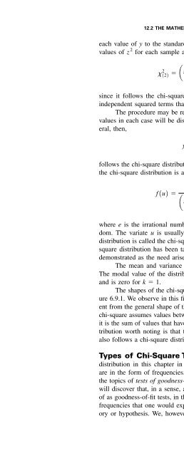
- Page 1214: 594 CHAPTER 12 THE CHI-SQUARE DISTR
- Page 1220: e equal to zero for each pair of ob
- Page 1224: 12.3 TESTS OF GOODNESS-OF-FIT 599 3
- Page 1228: 12.3 TESTS OF GOODNESS-OF-FIT 601 C
- Page 1232: 12.3 TESTS OF GOODNESS-OF-FIT 603 W
- Page 1236: 12.3 TESTS OF GOODNESS-OF-FIT 605 E
- Page 1240: 12.3 TESTS OF GOODNESS-OF-FIT 607 E
- Page 1244: 12.3 TESTS OF GOODNESS-OF-FIT 609 u
- Page 1248: EXERCISES 611 Test the goodness-of-
- Page 1252: a n 1. n ban .1 n b 12.4 TESTS OF I
- Page 1256: 12.4 TESTS OF INDEPENDENCE 615 3. H
- Page 1260: 12.4 TESTS OF INDEPENDENCE 617 The
- Page 1264: 12.4 TESTS OF INDEPENDENCE 619 EXAM
- Page 1268:
EXERCISES 621 EXERCISES In the exer
- Page 1272:
12.5 TESTS OF HOMOGENEITY 623 Polic
- Page 1276:
12.5 TESTS OF HOMOGENEITY 625 data,
- Page 1280:
EXERCISES 627 If we wish to test th
- Page 1284:
12.6 THE FISHER EXACT TEST 629 12.5
- Page 1288:
, A - a, and B - b are all greater
- Page 1292:
EXERCISES 633 Pl * Remained Cross-T
- Page 1296:
12.7 RELATIVE RISK, ODDS RATIO, AND
- Page 1300:
12.7 RELATIVE RISK, ODDS RATIO, AND
- Page 1304:
12.7 RELATIVE RISK, ODDS RATIO, AND
- Page 1308:
12.7 RELATIVE RISK, ODDS RATIO, AND
- Page 1312:
12.7 RELATIVE RISK, ODDS RATIO, AND
- Page 1316:
12.7 RELATIVE RISK, ODDS RATIO, AND
- Page 1320:
EXERCISES 647 12.7.2 The objective
- Page 1324:
12.8 SURVIVAL ANALYSIS 649 (3) the
- Page 1328:
12.8 SURVIVAL ANALYSIS 651 techniqu
- Page 1332:
12.8 SURVIVAL ANALYSIS 653 TABLE 12
- Page 1336:
cumulative proportion changes from
- Page 1340:
12.8 SURVIVAL ANALYSIS 657 TABLE 12
- Page 1344:
12.8 SURVIVAL ANALYSIS 659 Means an
- Page 1348:
EXERCISES 661 EXERCISES 12.8.1 Fift
- Page 1352:
EXERCISES 663 (c) Explain the meani
- Page 1356:
SUMMARY OF FORMULAS FOR CHAPTER 12
- Page 1360:
REVIEW QUESTIONS AND EXERCISES 667
- Page 1364:
REVIEW QUESTIONS AND EXERCISES 669
- Page 1368:
REVIEW QUESTIONS AND EXERCISES 671
- Page 1372:
REVIEW QUESTIONS AND EXERCISES 673
- Page 1376:
REVIEW QUESTIONS AND EXERCISES 675
- Page 1380:
REVIEW QUESTIONS AND EXERCISES 677
- Page 1384:
REFERENCES 679 19. WENDELL E. CARR,
- Page 1388:
A-30. A-31. A-32. A-33. A-34. A-35.
- Page 1392:
CHAPTER13 NONPARAMETRIC AND DISTRIB
- Page 1396:
13.2 MEASUREMENT SCALES 685 measure
- Page 1400:
13.3 THE SIGN TEST 687 TABLE 13.3.1
- Page 1404:
13.3 THE SIGN TEST 689 7. Calculati
- Page 1408:
13.3 THE SIGN TEST 691 TABLE 13.3.4
- Page 1412:
EXERCISES 693 Data: C1: 4 5 8 8 9 6
- Page 1416:
13.4 THE WILCOXON SIGNED-RANK TEST
- Page 1420:
13.4 THE WILCOXON SIGNED-RANK TEST
- Page 1424:
13.5 THE MEDIAN TEST 699 Subject 1
- Page 1428:
13.5 THE MEDIAN TEST 701 TABLE 13.5
- Page 1432:
13.6 THE MANN-WHITNEY TEST 703 Woul
- Page 1436:
13.6 THE MANN-WHITNEY TEST 705 TABL
- Page 1440:
13.6 THE MANN-WHITNEY TEST 707 FIGU
- Page 1444:
EXERCISES 709 Mann-Whitney-Wilcoxon
- Page 1448:
13.7 THE KOLMOGOROV-SMIRNOV GOODNES
- Page 1452:
13.7 THE KOLMOGOROV-SMIRNOV GOODNES
- Page 1456:
13.7 THE KOLMOGOROV-SMIRNOV GOODNES
- Page 1460:
13.8 THE KRUSKAL-WALLIS ONE-WAY ANA
- Page 1464:
13.8 THE KRUSKAL-WALLIS ONE-WAY ANA
- Page 1468:
13.8 THE KRUSKAL-WALLIS ONE-WAY ANA
- Page 1472:
EXERCISES 723 Young (19-50 Years) S
- Page 1476:
13.9 THE FRIEDMAN TWO-WAY ANALYSIS
- Page 1480:
13.9 THE FRIEDMAN TWO-WAY ANALYSIS
- Page 1484:
EXERCISES 729 Dialog box: Stat ➤
- Page 1488:
13.10 THE SPEARMAN RANK CORRELATION
- Page 1492:
13.10 THE SPEARMAN RANK CORRELATION
- Page 1496:
13.10 THE SPEARMAN RANK CORRELATION
- Page 1500:
EXERCISES 737 Dialog box: Stat ➤
- Page 1504:
EXERCISES 739 Duration of Follow-Up
- Page 1508:
13.11 NONPARAMETRIC REGRESSION ANAL
- Page 1512:
13.12 SUMMARY 743 36.4046 59.15 39.
- Page 1516:
REVIEW QUESTIONS AND EXERCISES 745
- Page 1520:
REVIEW QUESTIONS AND EXERCISES 747
- Page 1524:
REVIEW QUESTIONS AND EXERCISES 749
- Page 1528:
REVIEW QUESTIONS AND EXERCISES 751
- Page 1532:
REVIEW QUESTIONS AND EXERCISES 753
- Page 1536:
REVIEW QUESTIONS AND EXERCISES 755
- Page 1540:
REVIEW QUESTIONS AND EXERCISES 757
- Page 1544:
REVIEW QUESTIONS AND EXERCISES 759
- Page 1548:
REFERENCES 761 8. W. H. KRUSKAL and
- Page 1552:
CHAPTER14 VITAL STATISTICS CHAPTER
- Page 1556:
2. Ratio. A ratio is a fraction of
- Page 1560:
14.2 DEATH RATES AND RATIOS 767 TAB
- Page 1564:
14.2 DEATH RATES AND RATIOS 769 Som
- Page 1568:
EXERCISES 771 EXERCISES 14.2.1 The
- Page 1572:
14.3 MEASURES OF FERTILITY 773 1. C
- Page 1576:
EXERCISES 775 Age of Number of Birt
- Page 1580:
14.5 SUMMARY 777 4. Immaturity rati
- Page 1584:
REVIEW QUESTIONS AND EXERCISES 779
- Page 1588:
REVIEW QUESTIONS AND EXERCISES 781
- Page 1592:
REFERENCES 783 A-7. Georgia Divisio
- Page 1596:
APPENDIX STATISTICAL TABLES List of
- Page 1600:
APPENDIX STATISTICAL TABLES A-3 TAB
- Page 1604:
TABLE B (continued ) APPENDIX STATI
- Page 1608:
TABLE B (continued ) APPENDIX STATI
- Page 1612:
TABLE B (continued ) APPENDIX STATI
- Page 1616:
TABLE B (continued ) APPENDIX STATI
- Page 1620:
TABLE B (continued ) APPENDIX STATI
- Page 1624:
TABLE B (continued ) APPENDIX STATI
- Page 1628:
TABLE B (continued ) APPENDIX STATI
- Page 1632:
TABLE B (continued ) APPENDIX STATI
- Page 1636:
TABLE B (continued ) APPENDIX STATI
- Page 1640:
TABLE B (continued ) APPENDIX STATI
- Page 1644:
TABLE B (continued ) APPENDIX STATI
- Page 1648:
TABLE B (continued ) APPENDIX STATI
- Page 1652:
TABLE B (continued ) APPENDIX STATI
- Page 1656:
TABLE B (continued ) APPENDIX STATI
- Page 1660:
TABLE C (continued ) APPENDIX STATI
- Page 1664:
TABLE C (continued ) APPENDIX STATI
- Page 1668:
TABLE C (continued ) APPENDIX STATI
- Page 1672:
TABLE D (continued ) APPENDIX STATI
- Page 1676:
APPENDIX STATISTICAL TABLES A-41 TA
- Page 1680:
TABLE G (continued ) APPENDIX STATI
- Page 1684:
TABLE G (continued ) APPENDIX STATI
- Page 1688:
TABLE G (continued ) APPENDIX STATI
- Page 1692:
TABLE G (continued ) APPENDIX STATI
- Page 1696:
TABLE G (continued ) APPENDIX STATI
- Page 1700:
TABLE H (continued ) APPENDIX STATI
- Page 1704:
APPENDIX STATISTICAL TABLES A-55 TA
- Page 1708:
TABLE J (continued ) APPENDIX STATI
- Page 1712:
TABLE J (continued ) APPENDIX STATI
- Page 1716:
TABLE J (continued ) APPENDIX STATI
- Page 1720:
TABLE J (continued ) APPENDIX STATI
- Page 1724:
TABLE J (continued ) APPENDIX STATI
- Page 1728:
TABLE J (continued ) APPENDIX STATI
- Page 1732:
TABLE J (continued ) APPENDIX STATI
- Page 1736:
TABLE J (continued ) APPENDIX STATI
- Page 1740:
TABLE J (continued ) APPENDIX STATI
- Page 1744:
TABLE J (continued ) APPENDIX STATI
- Page 1748:
TABLE J (continued ) APPENDIX STATI
- Page 1752:
TABLE J (continued ) APPENDIX STATI
- Page 1756:
TABLE J (continued ) APPENDIX STATI
- Page 1760:
TABLE J (continued ) APPENDIX STATI
- Page 1764:
TABLE J (continued ) APPENDIX STATI
- Page 1768:
TABLE K (continued ) APPENDIX STATI
- Page 1772:
TABLE K (continued ) APPENDIX STATI
- Page 1776:
TABLE K (continued ) APPENDIX STATI
- Page 1780:
TABLE K (continued ) APPENDIX STATI
- Page 1784:
APPENDIX STATISTICAL TABLES A-95 TA
- Page 1788:
TABLE L (continued ) APPENDIX STATI
- Page 1792:
APPENDIX STATISTICAL TABLES A-99 TA
- Page 1796:
TABLE N (continued ) APPENDIX STATI
- Page 1800:
APPENDIX STATISTICAL TABLES A-103 T
- Page 1804:
APPENDIX STATISTICAL TABLES A-105 A
- Page 1808:
ANSWERS TO ODD-NUMBERED EXERCISES A
- Page 1812:
ANSWERS TO ODD-NUMBERED EXERCISES A
- Page 1816:
ANSWERS TO ODD-NUMBERED EXERCISES A
- Page 1820:
ANSWERS TO ODD-NUMBERED EXERCISES A
- Page 1824:
ANSWERS TO ODD-NUMBERED EXERCISES A
- Page 1828:
ANSWERS TO ODD-NUMBERED EXERCISES A
- Page 1832:
ANSWERS TO ODD-NUMBERED EXERCISES A
- Page 1836:
ANSWERS TO ODD-NUMBERED EXERCISES A
- Page 1840:
ANSWERS TO ODD-NUMBERED EXERCISES A
- Page 1844:
ANSWERS TO ODD-NUMBERED EXERCISES A
- Page 1848:
Family error rate = 0.0500 Individu
- Page 1852:
ANSWERS TO ODD-NUMBERED EXERCISES A
- Page 1856:
ANSWERS TO ODD-NUMBERED EXERCISES A
- Page 1860:
ANSWERS TO ODD-NUMBERED EXERCISES A
- Page 1864:
ANSWERS TO ODD-NUMBERED EXERCISES A
- Page 1868:
ANSWERS TO ODD-NUMBERED EXERCISES A
- Page 1872:
The regression equation is WL = 0.7
- Page 1876:
ANSWERS TO ODD-NUMBERED EXERCISES A
- Page 1880:
ANSWERS TO ODD-NUMBERED EXERCISES A
- Page 1884:
S 1.06 1.01 0.990 R-Sq 8.57 18.10 2
- Page 1888:
ANSWERS TO ODD-NUMBERED EXERCISES A
- Page 1892:
ANSWERS TO ODD-NUMBERED EXERCISES A
- Page 1896:
ANSWERS TO ODD-NUMBERED EXERCISES A
- Page 1900:
INDEX Numbers preceded by A refer t
- Page 1904:
INDEX I-3 H Histogram, 25-27 Hypoth
- Page 1908:
INDEX I-5 Rate, 764-765 Ratio, 765