Oasys LS-DYNA Environment 8.1 VOLUME 3 ... - Oasys Software

Oasys LS-DYNA Environment: User Guide (Version 8.1)
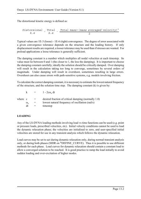
The distortional kinetic energy is defined as:
Distorsional
k.e
Total
k.e
Total mass (mass averaged velocity) 2
Typical values are 1E-3 (loose) - 1E-6 (tight) convergence. The degree of error associated with
a given convergence tolerance depends on the structure and the loading history. If only
displacement results are required, a looser tolerance may be used than if stresses are wanted. For
preload applications a loose tolerance is generally sufficient.
The damping constant is a number which multiplies all nodal velocities at each timestep. Its
value must lie between 0 and 1 (the closer to 1, the less the damping). It is important to choose
the damping constant carefully; ideally the solution should be critically damped. Over damping
will result in the calculation taking too long to converge, sometimes by several orders of
magnitude. Under damping will result in overshoot, sometimes resulting in large errors.
Overshoot can also cause errors with path-sensitive systems, e.g. models involving friction.
To calculate the correct damping constant, it is necessary to estimate the lowest natural frequency
of the structure, and the solution time step. The damping constant (k) is given by:
k = 1 - 2cω n dt
where c = desired fraction of critical damping (normally 1.0)
ω n = lowest natural frequency of oscillation (rad/s)
dt = timestep
LOADING
Any of the LS-DYNA loading methods involving load vs time functions can be used (e.g. point
or pressure loads, prescribed velocities, etc). Initial velocity conditions cannot be used to load
the dynamic relaxation phase; the velocities are initialised to zero, and user-specified initial
velocities are stored for use in any transient analysis which follows the dynamic relaxation.
Load curves may be set to act during dynamic relaxation only, during normal transient analysis
only, or during both phases (SIDR on *DEFINE_CURVE). Thus it is possible to use different
methods for each phase. Load curves for dynamic relaxation should contain a constant load to
allow a converged solution to be reached. It is good practice to ramp the load initially to avoid
sudden loading and over-excitation of higher modes.
2
Page 13.2