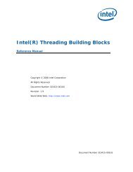
4.2. GRAPH COMMANDS (IN DETAIL) 25begin graphxtitle "Age"ytitle "Weight"data "age.csv"key pos br compactd1 line color red marker circled2 line color blue marker triangled3 line color green marker squareend graphAge, John, Mary, Ken15, 73, 65, 7720, 80, 68, 7730, 82, 76, 8040, 85, 77, 82Weight8580757065JohnMaryKen15 20 25 30 35 40AgeFigure 4.1: Line graph with key taken from the column labels in the first data row. Left: the graphblock; middle: the dataset “age.csv”; right: the resulting graph.1, 2.7, 32, 5, *3, 7.8, 74, 9, 4The first point of dataset d1 would then be (1, 2.7) and the first point of dataset d2 would be (1,3). The data values can be space, tab, comma, or semi-colon separated.Missing values can be indicated with “*”, “?”, “-”, or “.”.The option d3=c2,c3 allows particular columns of data to be read into a dataset. In this example,d3 would read its x-values from column 2 and y-values from column 3.size 7 3.5begin graphsize 6 3title "Simple Graph"xtitle "Time"ytitle "Output"data "data.csv"d1 line marker triangle color redend graphOutput108642Simple Graph01.0 1.5 2.0 2.5 3.0 3.5 4.0 4.5 5.0TimeComments: Comments can be included with the symbol “!”. All characters from “!” until theend of the line of the data file are ignored. It is possible to change the symbol that indicates acomment with the option ‘comment’. E.g., with ‘data "data.csv" comment #’, lines starting with# will be treated as comments.Ignore header: The option ignore n makes <strong>GLE</strong> ignore the first n lines of the data file. This isuseful if the first n lines do not contain data.Auto key: If the first row of a data file does not contain actual data but instead contains columnlabels, then these labels are used by <strong>GLE</strong> to create a key for the graph (Chapter 5). <strong>GLE</strong> automaticallydetects this case by checking if all fields in the first row are valid numbers or not. If not,then <strong>GLE</strong> assumes that the first row contains column labels. Column labels that include a spaceor that could be incorrectly interpreted as a number should be double quoted. Fig. 4.1 illustratesthis with an example.Auto x-labels: If the first column of a data file does not contain numeric data, but instead containssymbolic labels, then these labels are used to label the horizontal axis. For example, if the data filecontainsMon, 1Tue, 4Wed, 3.5Thu, 2Fri, 1Sat, 5Sun, 4
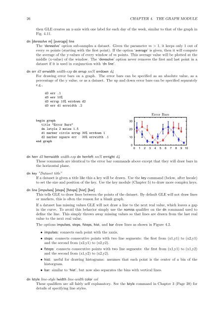
26 CHAPTER 4. THE GRAPH MODULEthen <strong>GLE</strong> creates an x-axis with one label for each day of the week, similar to that of the graph inFig. 4.11.dn [deresolve m] [average] lineThe ‘deresolve’ option sub-samples a dataset. Given the parameter m > 1, it keeps only 1 out ofevery m points (starting with the first point). If the option ‘average’ is given, then it will computethe average of the y-values of every window of m points. This average value will be plotted at themiddle (x-value) of the window. The ‘deresolve’ option never removes the first and last point in adataset if it is used in conjunction with ‘dn line’.dn err d5 errwidth width-exp dn errup nn% errdown d4For drawing error bars on a graph. The error bars can be specified as an absolute value, as apercentage of the y value, or as a dataset. The up and down error bars can be specified separatelye.g.,d3 err .1d3 err 10%d3 errup 10% errdown d2d3 err d1 errwidth .2begin graphtitle "Error Bars"dn lstyle 2 msize 1.5d1 marker circle errup 30% errdown 1d2 marker square err 30% errwidth .1end graphError Bars30201000 1 2 3 4 5 6 7 8 9 10dn herr d5 herrwidth width-exp dn herrleft nn% errright d4These commands are identical to the error bar commands above except that they will draw bars inthe horizontal plane.dn key ”Dataset title”If a dataset is given a title like this a key will be drawn. Use the key command (below, after hscale)to set the size and position of the key. Use the key module (Chapter 5) to draw more complex keys.dn line [impulses] [steps] [fsteps] [hist] [bar]This tells <strong>GLE</strong> to draw lines between the points of the dataset. By default <strong>GLE</strong> will not draw linesor markers, this is often the reason for a blank graph.If a dataset has missing values <strong>GLE</strong> will not draw a line to the next real value, which leaves a gapin the curve. To avoid this behavior simply use the nomiss qualifier on the dn command used todefine the line. This simply throws away missing values so that lines are drawn from the last realvalue to the next real value.The options impulses, steps, fsteps, hist, and bar draw lines as shown in Figure 4.2.• impulses: connects each point with the xaxis.• steps: connects consecutive points with two line segments: the first from (x1,y1) to (x2,y1)and the second from (x2,y1) to (x2,y2).• fsteps: connects consecutive points with two line segments: the first from (x1,y1) to (x1,y2)and the second from (x1,y2) to (x2,y2).• hist: useful for drawing histograms: assumes that each point is the center of a bin of thehistorgram.• bar: similar to ‘hist’, but now also separates the bins with vertical lines.dn lstyle line-style lwidth line-width color colThese qualifiers are all fairly self explanatory. See the lstyle command in Chapter 3 (Page 20) fordetails of specifying line styles.
- Page 1: Professional Graphics LanguageProfe
- Page 4 and 5: ivCONTENTS7.2.4 Import a GLE Figure
- Page 6 and 7: 1• Chapter 4, The Graph Module:De
- Page 8 and 9: Chapter 2Tutorial2.1 Installing GLE
- Page 10 and 11: 2.4. DRAWING A SIMPLE GRAPH 5gle -p
- Page 12 and 13: Chapter 3PrimitivesA GLE command is
- Page 14 and 15: 3.2. GRAPHICS PRIMITIVES (IN DETAIL
- Page 16 and 17: 3.2. GRAPHICS PRIMITIVES (IN DETAIL
- Page 18 and 19: 3.2. GRAPHICS PRIMITIVES (IN DETAIL
- Page 20 and 21: 3.2. GRAPHICS PRIMITIVES (IN DETAIL
- Page 22 and 23: 3.2. GRAPHICS PRIMITIVES (IN DETAIL
- Page 24 and 25: 3.2. GRAPHICS PRIMITIVES (IN DETAIL
- Page 26 and 27: 3.2. GRAPHICS PRIMITIVES (IN DETAIL
- Page 28 and 29: Chapter 4The Graph ModuleA graph sh
- Page 32 and 33: 4.2. GRAPH COMMANDS (IN DETAIL) 271
- Page 34 and 35: 4.2. GRAPH COMMANDS (IN DETAIL) 29M
- Page 36 and 37: 4.2. GRAPH COMMANDS (IN DETAIL) 31a
- Page 38 and 39: 4.2. GRAPH COMMANDS (IN DETAIL) 33x
- Page 40 and 41: 4.2. GRAPH COMMANDS (IN DETAIL) 351
- Page 42 and 43: 4.3. BAR GRAPHS 37Planet sizesNeptu
- Page 44 and 45: 4.6. NOTES ON DRAWING GRAPHS 394.6
- Page 46 and 47: Chapter 5The Key ModuleThe key modu
- Page 48 and 49: 5.2. ENTRY DEFINITION COMMANDS 43ju
- Page 50 and 51: 5.3. DEFINING THE KEY IN THE GRAPH
- Page 52 and 53: Chapter 6Programming Facilities6.1
- Page 54 and 55: 6.2. FUNCTIONS INSIDE EXPRESSIONS 4
- Page 56 and 57: 6.5. IF-THEN-ELSE 51Besides for-nex
- Page 58 and 59: 6.9. DEVICE DEPENDEND CONTROL 53fwr
- Page 60 and 61: Chapter 7Advanced FeaturesThis chap
- Page 62 and 63: 7.1. DIAGRAMS 57GRVCheeseCHVGoatsMa
- Page 64 and 65: 7.2. L A TEX INTERFACE 59house.wind
- Page 66 and 67: 7.4. COLOUR 61size 10 5begin clip !
- Page 68 and 69: Chapter 8Surface and Contour Plots8
- Page 70 and 71: 8.1. SURFACE PRIMITIVES 65ylines of
- Page 72 and 73: 8.2. LETZ 67zclip [min v1 ] [max v2
- Page 74 and 75: 8.5. COLOR MAPS 69• pixels-x, pix
- Page 76 and 77: Chapter 9GLE Utilities9.1 FitlsThe
- Page 78 and 79: 9.2. MANIP 73c1 == c1c1r1r10 == 1,1
- Page 80 and 81:
9.2. MANIP 75BLANK"% BLANK C2C3" Cl
- Page 82 and 83:
9.2. MANIP 77PARSUM [range1] [range
- Page 84 and 85:
Appendix ATablesA.1 Markerstriangle
- Page 86 and 87:
A.2. FUNCTIONS AND VARIABLES 81widt
- Page 88 and 89:
A.4. INSTALLING GLE 83A.4 Installin
- Page 90 and 91:
A.6. FONT TABLES 85Typewriter (tt)0
- Page 92 and 93:
A.6. FONT TABLES 87TEXComputer Mode
- Page 94 and 95:
A.6. FONT TABLES 89PostScript Helve
- Page 96 and 97:
A.6. FONT TABLES 91(psbl)0246810121
- Page 98 and 99:
A.6. FONT TABLES 93PostScript ZapfC
- Page 100 and 101:
A.7. PREDEFINED COLORS 95GLE suppor
- Page 102 and 103:
Index!, 8, 25\expr(exp), 80.z file,
- Page 104 and 105:
INDEX 99histogram, 30horiz, 37horiz
- Page 106:
INDEX 101under, 32underneath, 66Uni