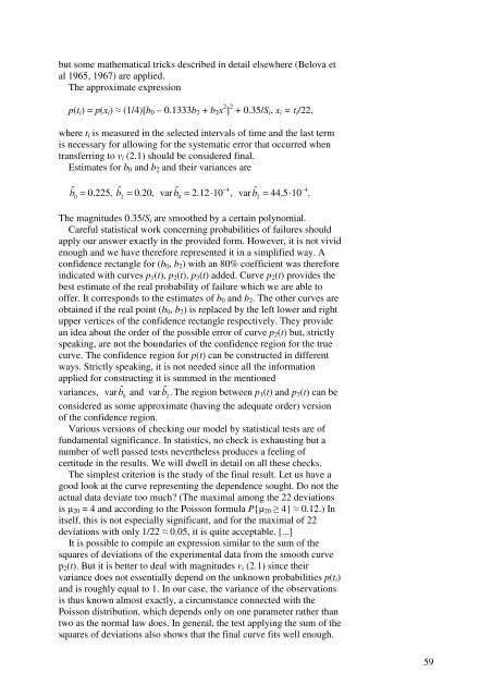
<strong>the</strong> <strong>in</strong>crease <strong>of</strong> <strong>the</strong> probability <strong>of</strong> failure with time, was formulated.[...]The values <strong>of</strong> <strong>the</strong> frequencies <strong>of</strong> failures comprise a broken l<strong>in</strong>e.Their scatter <strong>in</strong>creases with t, a circumstance connected with a sharpdecrease <strong>of</strong> <strong>the</strong> area <strong>of</strong> <strong>in</strong>sulation, i. e., <strong>of</strong> <strong>the</strong> amount <strong>of</strong> experimentalmaterial.We are <strong>in</strong>terested <strong>in</strong> <strong>the</strong> values <strong>of</strong> probabilities p(t) <strong>of</strong> a failure <strong>of</strong> aunit area <strong>of</strong> <strong>in</strong>sulation aged t dur<strong>in</strong>g unit time (10 4 work<strong>in</strong>g hours,about 1.5 years). For small values <strong>of</strong> t <strong>the</strong> amount <strong>of</strong> experimentalmaterial is large, but p(t) <strong>the</strong>mselves are low, 0.01 – 0.02, so that <strong>the</strong>irdirect determ<strong>in</strong>ation through frequencies is fraught with very largeerrors. The mean square deviation <strong>of</strong> <strong>the</strong> frequency, µ i /S i , where µ i is<strong>the</strong> number <strong>of</strong> failures dur<strong>in</strong>g time <strong>in</strong>terval between (i – 1)-th <strong>and</strong> i-thtime units <strong>and</strong> S i , <strong>the</strong> correspond<strong>in</strong>g area <strong>of</strong> <strong>in</strong>sulation, is known to beequal top( ti)[1 − p( ti)]Siwhere t i =10 4 i hours. For t 1 = 10 5 p(t i ) ≈ 0.02, S i = 200, so thatdeviation is roughly 0.01 or 50% <strong>of</strong> p(t) itself.Then it is natural to attempt to heighten <strong>the</strong> precision <strong>of</strong> determ<strong>in</strong><strong>in</strong>gp(t) by smooth<strong>in</strong>g s<strong>in</strong>ce <strong>the</strong> estimation <strong>of</strong> this probability <strong>the</strong>n dependson all o<strong>the</strong>r experimental data. But <strong>the</strong>n, a statistical model isnecessary here. It is ra<strong>the</strong>r natural to consider <strong>the</strong> observed number <strong>of</strong>failures (1.2) as r<strong>and</strong>om variables with a Poisson distribution.Underst<strong>and</strong>ably,Eµ i = S i p(t i ).It is somewhat more difficult to agree that <strong>the</strong> magnitudes µ i are<strong>in</strong>dependent. Here, however, <strong>the</strong> follow<strong>in</strong>g considerations applicableto any rare events will help. Take for example µ 1 , µ 2 . Failure occurr<strong>in</strong>gdur<strong>in</strong>g <strong>the</strong> first <strong>in</strong>terval <strong>of</strong> time <strong>in</strong>fluences <strong>the</strong> behaviour <strong>of</strong> <strong>the</strong><strong>in</strong>sulation <strong>in</strong> <strong>the</strong> second <strong>in</strong>terval, but that action is only restricted to <strong>the</strong>failed mach<strong>in</strong>es whose portion was small. Hav<strong>in</strong>g admitted<strong>in</strong>dependence, <strong>the</strong> ma<strong>the</strong>matical model is completely given although itis connected not with <strong>the</strong> most convenient normal, but with <strong>the</strong>Poisson distribution. Then, <strong>the</strong> variancesvar µ i = Eµ i = S i p(t i )depend on probabilities p(t i ) which we <strong>in</strong>deed aim to derive. Atransformation to magnitudesv = 2 µ(2.1)iiessentially equalizes <strong>the</strong> variances <strong>and</strong> <strong>the</strong>refore helps.These magnitudes v 1 , v 2 , ..., v n from which we later return tomagnitudes (1.2) are smoo<strong>the</strong>d. The smooth<strong>in</strong>g itself is easy <strong>in</strong> essence58
ut some ma<strong>the</strong>matical tricks described <strong>in</strong> detail elsewhere (Belova etal 1965, 1967) are applied.The approximate expressionp(t i ) = p(x i ) ≈ (1/4)[b 0 – 0.1333b 2 + b 2 x 2 ] 2 + 0.35/S i , x i = t i /22,where t i is measured <strong>in</strong> <strong>the</strong> selected <strong>in</strong>tervals <strong>of</strong> time <strong>and</strong> <strong>the</strong> last termis necessary for allow<strong>in</strong>g for <strong>the</strong> systematic error that occurred whentransferr<strong>in</strong>g to v i (2.1) should be considered f<strong>in</strong>al.Estimates for b 0 <strong>and</strong> b 2 <strong>and</strong> <strong>the</strong>ir variances arebˆ = 0.225, bˆ = 0.20, var bˆ = 2.12⋅ 10 , var bˆ= 44.5⋅10 .−4 −40 2 0 2The magnitudes 0.35/S i are smoo<strong>the</strong>d by a certa<strong>in</strong> polynomial.Careful statistical work concern<strong>in</strong>g probabilities <strong>of</strong> failures shouldapply our answer exactly <strong>in</strong> <strong>the</strong> provided form. However, it is not vividenough <strong>and</strong> we have <strong>the</strong>refore represented it <strong>in</strong> a simplified way. Aconfidence rectangle for (b 0 , b 2 ) with an 80% coefficient was <strong>the</strong>refore<strong>in</strong>dicated with curves p 1 (t), p 2 (t), p 3 (t) added. Curve p 2 (t) provides <strong>the</strong>best estimate <strong>of</strong> <strong>the</strong> real probability <strong>of</strong> failure which we are able to<strong>of</strong>fer. It corresponds to <strong>the</strong> estimates <strong>of</strong> b 0 <strong>and</strong> b 2 . The o<strong>the</strong>r curves areobta<strong>in</strong>ed if <strong>the</strong> real po<strong>in</strong>t (b 0 , b 2 ) is replaced by <strong>the</strong> left lower <strong>and</strong> rightupper vertices <strong>of</strong> <strong>the</strong> confidence rectangle respectively. They providean idea about <strong>the</strong> order <strong>of</strong> <strong>the</strong> possible error <strong>of</strong> curve p 2 (t) but, strictlyspeak<strong>in</strong>g, are not <strong>the</strong> boundaries <strong>of</strong> <strong>the</strong> confidence region for <strong>the</strong> truecurve. The confidence region for p(t) can be constructed <strong>in</strong> differentways. Strictly speak<strong>in</strong>g, it is not needed s<strong>in</strong>ce all <strong>the</strong> <strong>in</strong>formationapplied for construct<strong>in</strong>g it is summed <strong>in</strong> <strong>the</strong> mentionedvariances, var bˆˆ0<strong>and</strong> var b2.The region between p 1 (t) <strong>and</strong> p 3 (t) can beconsidered as some approximate (hav<strong>in</strong>g <strong>the</strong> adequate order) version<strong>of</strong> <strong>the</strong> confidence region.Various versions <strong>of</strong> check<strong>in</strong>g our model by statistical tests are <strong>of</strong>fundamental significance. In statistics, no check is exhaust<strong>in</strong>g but anumber <strong>of</strong> well passed tests never<strong>the</strong>less produces a feel<strong>in</strong>g <strong>of</strong>certitude <strong>in</strong> <strong>the</strong> results. We will dwell <strong>in</strong> detail on all <strong>the</strong>se checks.The simplest criterion is <strong>the</strong> study <strong>of</strong> <strong>the</strong> f<strong>in</strong>al result. Let us have agood look at <strong>the</strong> curve represent<strong>in</strong>g <strong>the</strong> dependence sought. Do not <strong>the</strong>actual data deviate too much? (The maximal among <strong>the</strong> 22 deviationsis µ 20 = 4 <strong>and</strong> accord<strong>in</strong>g to <strong>the</strong> Poisson formula P{µ 20 ≥ 4} ≈ 0.12.) Initself, this is not especially significant, <strong>and</strong> for <strong>the</strong> maximal <strong>of</strong> 22deviations with only 1/22 ≈ 0.05, it is quite acceptable. [...]It is possible to compile an expression similar to <strong>the</strong> sum <strong>of</strong> <strong>the</strong>squares <strong>of</strong> deviations <strong>of</strong> <strong>the</strong> experimental data from <strong>the</strong> smooth curvep 2 (t). But it is better to deal with magnitudes v i (2.1) s<strong>in</strong>ce <strong>the</strong>irvariance does not essentially depend on <strong>the</strong> unknown probabilities p(t i )<strong>and</strong> is roughly equal to 1. In our case, <strong>the</strong> variance <strong>of</strong> <strong>the</strong> observationsis thus known almost exactly, a circumstance connected with <strong>the</strong>Poisson distribution, which depends only on one parameter ra<strong>the</strong>r thantwo as <strong>the</strong> normal law does. In general, <strong>the</strong> test apply<strong>in</strong>g <strong>the</strong> sum <strong>of</strong> <strong>the</strong>squares <strong>of</strong> deviations also shows that <strong>the</strong> f<strong>in</strong>al curve fits well enough.59
- Page 1 and 2:
Studies in the History of Statistic
- Page 3 and 4:
Introduction by CompilerI am presen
- Page 5 and 6:
(Lect. Notes Math., No. 1021, 1983,
- Page 7 and 8: sufficiently securely that a carefu
- Page 9 and 10: is energy?) from chapter 4 of Feynm
- Page 11 and 12: demand to apply transfinite numbers
- Page 13 and 14: for stating that Ω consists of ele
- Page 15 and 16: chances to draw a more suitable apa
- Page 17 and 18: Let the space of elementary events
- Page 19 and 20: 2.3. Independence. When desiring to
- Page 21 and 22: Eξ = ∑ aipi.Our form of definiti
- Page 23 and 24: absolutely precisely if the pertine
- Page 25 and 26: where x is any real number. If dens
- Page 27 and 28: probability can be coupled with an
- Page 29 and 30: Nowadays we are sure that no indepe
- Page 31 and 32: λ = λ(T)with λ(T) being actually
- Page 33 and 34: (1/B n )(m − A n )instead of the
- Page 35 and 36: along with ξ. For example, if ξ i
- Page 37 and 38: µ( − p0) ÷np0 (1 − p0)nhas an
- Page 39 and 40: distribution of the maximal term |s
- Page 41 and 42: ξ (ω) + ... + ξ (ω)n1n{ω :|
- Page 43 and 44: P{max ξ(t) ≥ x} = 0.01, 0 ≤ t
- Page 45 and 46: 1. This example and considerations
- Page 47 and 48: IIV. N. TutubalinTreatment of Obser
- Page 49 and 50: structure of statistical methods, d
- Page 51 and 52: Suppose that we have adopted the pa
- Page 53 and 54: and the variances are inversely pro
- Page 55 and 56: It is interesting therefore to see
- Page 57: is applied with P(t) being a polyno
- Page 61 and 62: It is clear therefore that no speci
- Page 63 and 64: of various groups of machines, and
- Page 65 and 66: nnA(λ) x sin λ t, B(λ) = x cosλ
- Page 67 and 68: of the mathematical model of the Br
- Page 69 and 70: dF(λ) = f (λ) dλ, so that B( t
- Page 71 and 72: usually very little of them. Indeed
- Page 73 and 74: This is the celebrated model of aut
- Page 75 and 76: applications of the theory of stoch
- Page 77 and 78: achieved by differentiating because
- Page 79 and 80: u(x 1 , x 2 , t 1 , t 2 ) = v(x 1 ,
- Page 81 and 82: Reasoning based on common sense and
- Page 83 and 84: answering that question is extremel
- Page 85 and 86: IIIV. N. TutubalinThe Boundaries of
- Page 87 and 88: periodograms. It occurred that work
- Page 89 and 90: at point x = 1. However, preceding
- Page 91 and 92: He concludes that since the action
- Page 93 and 94: The verification of the truth of a
- Page 95 and 96: In the purely scientific sense this
- Page 97 and 98: ought to learn at once the simple t
- Page 99 and 100: the material world science had inde
- Page 101 and 102: values of (2.1) realized in the n e
- Page 103 and 104: *several dozen. The totality µ ica
- Page 105 and 106: Mendelian laws. It is not sufficien
- Page 107 and 108: example, the problem of the objecti
- Page 109 and 110:
a linear function is not restricted
- Page 111 and 112:
258 - 82 - 176 cases or 68.5% of al
- Page 113 and 114:
The Framingham investigation indeed
- Page 115 and 116:
or, for discrete observations,IT(ω
- Page 117 and 118:
What objections can be made? First,
- Page 119 and 120:
eliability and queuing are known to
- Page 121 and 122:
Kolman E. (1939 Russian), Perversio
- Page 123 and 124:
measurement is provided. Recently,
- Page 125 and 126:
which means that sooner or later th
- Page 127 and 128:
The foundations of the Mises approa
- Page 129 and 130:
A rather subtle arsenal is develope
- Page 131 and 132:
4.3. General remarks on §§ 4.1 an
- Page 133 and 134:
BibliographyAlimov Yu. I. (1976, 19
- Page 135 and 136:
processes are now going on in the s
- Page 137 and 138:
obtaining a deviation from the theo
- Page 139 and 140:
VIOscar SheyninOn the Bernoulli Law