TESIS
TESIS
TESIS

Create successful ePaper yourself
Turn your PDF publications into a flip-book with our unique Google optimized e-Paper software.
σ<br />
m<br />
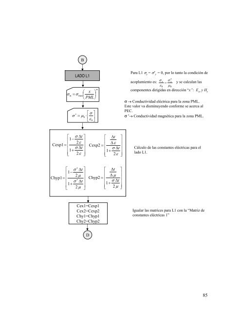
B<br />
LADO L1<br />
= σ max<br />
⎡ σ ∆t<br />
⎤<br />
⎢<br />
1−<br />
2ε<br />
⎥<br />
Cexp1 = ⎢ ⎥<br />
⎢ σ ∆t<br />
1+<br />
⎥<br />
⎢⎣<br />
2ε<br />
⎥⎦<br />
Chyp1<br />
⎛ x ⎞<br />
⎜ ⎟⎠<br />
⎝ PML<br />
Para L1 σy = σ * y = 0, por lo tanto la condición de<br />
∗<br />
acoplamiento es:<br />
σ σ<br />
= y se calculan las<br />
ε 0 µ 0<br />
componentes dirigidas en dirección “x”: Ezx y Hy x x<br />
σ → Conductividad eléctrica para la zona PML.<br />
Este valor va disminuyendo conforme se acerca al<br />
PEC.<br />
∗ ⎡ σ ⎤<br />
σ = µ 0 ⋅ ⎢ ⎥<br />
σ<br />
⎣ε<br />
0 ⎦<br />
* → Conductividad magnética para la zona PML.<br />
D<br />
m<br />
⎡ ∆t<br />
⎤<br />
⎢ ∆ε<br />
⎥<br />
Cexp2 = ⎢ ⎥<br />
⎢ σ ∆t<br />
1+<br />
⎥<br />
⎢⎣<br />
2ε<br />
⎥⎦<br />
∗ ⎡ σ ∆t<br />
⎤ ⎡ ∆t<br />
⎤<br />
⎢1−<br />
⎥<br />
⎢<br />
2 µ<br />
⎢ ∆ µ ⎥<br />
⎥ Chyp2 = ⎢ ⎥<br />
⎢ σ ∆t<br />
⎥<br />
⎢<br />
1+<br />
⎢ σ ∆t<br />
1+<br />
⎥<br />
⎥<br />
⎣ 2 µ<br />
⎢ ⎥<br />
⎦ ⎣ 2 µ ⎦<br />
= ∗<br />
Cex1=Cexp1<br />
Cex2=Cexp2<br />
Chy1=Chyp1<br />
Chy2=Chyp2<br />
Cálculo de las constantes eléctricas para el<br />
lado L1.<br />
Igualar las matrices para L1 con la “Matriz de<br />
constantes eléctricas 1”<br />
85