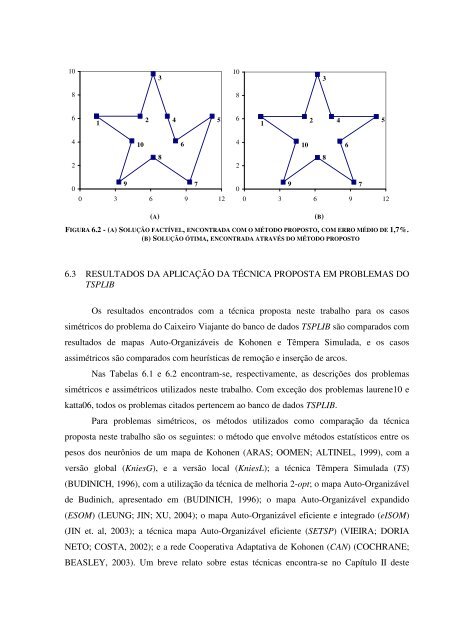
⎛ 0 ⎜ ⎜0, 2630 ⎜0, 2334 ⎜ ⎜0, 0013 ⎜ = ⎜ 0, 0004 x ⎜ 0, 0001 ⎜ ⎜0, 0004 ⎜0, 0017 ⎜ ⎜0, 2213 ⎜ ⎝0, 2783 0, 2557 0 0, 2722 0, 2114 0, 0058 0, 0093 0, 0011 0, 0095 0, 0071 0, 2279 0, 2436 0, 2744 0 0, 2649 0, 2125 0, 0016 0, 0005 0, 0001 0, 0005 0, 0019 0, 0063 0, 2062 0, 2669 0 0, 2492 0, 2445 0, 0074 0, 0092 0, 0011 0, 0094 0, 0004 0, 0011 0, 2108 0, 2511 0 0, 2723 0, 2624 0, 0014 0, 0004 0 0, 0011 0, 0094 0, 0072 0, 2508 0, 2650 0 0, 2655 0, 1860 0, 0065 0, 0083 0, 0004 0 0, 0005 0, 0017 0, 2597 0, 2717 0 0, 2613 0, 2031 0, 0013 0, 0073 0, 0097 0, 0011 0, 0093 0, 0061 0, 1907 0, 2608 0 0, 3037 0, 2116 0, 2198 0, 0017 0, 0005 0, 0001 0, 0004 0, 0014 0, 1963 0, 3189 0 0, 2614 0, 2654⎞ ⎟ 0, 2345⎟ 0, 0074⎟ ⎟ 0, 0094⎟ 0, 0010 ⎟ ⎟ 0, 0083⎟ ⎟ 0, 0059⎟ 0, 2120⎟ ⎟ 0, 2562⎟ 0 ⎟ ⎠ Através <strong>do</strong> princípio Winner Takes All, <strong>uma</strong> aproximação para a solução ótima deste <strong>problema</strong> é encontrada, com a rota: x ~ = (10, 1, 2, 3, 4, 5, 6, 7, 8, 9, 10), com custo de 37,159 (Figura 6.2B). ⎛ 0 ⎜ ⎜ 0 ⎜ 0 ⎜ ⎜ 0 ⎜ ⎜ 0 x = ⎜ 0 ⎜ ⎜ 0 ⎜ 0 ⎜ ⎜ 0 ⎜ ⎝1, 0001 1, 0002 0 0 0 0 0 0 0 0 0 0 0, 9999 0 0 0 0 0 0 0 0 0 0 1, 0002 0 0 0 0 0 0 0 0 1, 0001 0 0 0 0 0 0 0 0 0, 9998 0 0 0 0 0 0 0 0 1 0 0 0 0 0 0 0 0 0, 9999 Na próxima seção são mostra<strong>do</strong>s os resulta<strong>do</strong>s da aplicação desta técnica para alguns <strong>problema</strong>s <strong>do</strong> TSPLIB, tanto para <strong>problema</strong>s simétricos quanto assimétricos. 0 0 0 0 0 0 0 0 0 0 0 0 0 0 0 0 0 0 1 0 0 0⎞ ⎟ 0⎟ 0⎟ ⎟ 0⎟ 0 ⎟ ⎟ 0⎟ ⎟ 0⎟ 0⎟ ⎟ 1⎟ 0 ⎟ ⎠
10 8 6 4 2 0 1 10 2 3 8 9 7 0 3 6 9 12 4 6 5 10 8 6 4 2 0 1 9 10 3 2 4 5 0 3 6 9 12 (A) (B) FIGURA 6.2 - (A) SOLUÇÃO FACTÍVEL, ENCONTRADA COM O MÉTODO PROPOSTO, COM ERRO MÉDIO DE 1,7%. (B) SOLUÇÃO ÓTIMA, ENCONTRADA ATRAVÉS DO MÉTODO PROPOSTO 6.3 RESULTADOS DA APLICAÇÃO DA TÉCNICA PROPOSTA EM PROBLEMAS DO TSPLIB Os resulta<strong>do</strong>s encontra<strong>do</strong>s com a técnica proposta neste trabalho para os casos simétricos <strong>do</strong> <strong>problema</strong> <strong>do</strong> Caixeiro Viajante <strong>do</strong> banco de da<strong>do</strong>s TSPLIB são compara<strong>do</strong>s com resulta<strong>do</strong>s de mapas Auto-Organizáveis de Kohonen e Têmpera Simulada, e os casos assimétricos são compara<strong>do</strong>s com heurísticas de remoção e inserção de arcos. Nas Tabelas 6.1 e 6.2 encontram-se, respectivamente, as descrições <strong>do</strong>s <strong>problema</strong>s simétricos e assimétricos utiliza<strong>do</strong>s neste trabalho. Com exceção <strong>do</strong>s <strong>problema</strong>s laurene10 e katta06, to<strong>do</strong>s os <strong>problema</strong>s cita<strong>do</strong>s pertencem ao banco de da<strong>do</strong>s TSPLIB. Para <strong>problema</strong>s simétricos, os méto<strong>do</strong>s utiliza<strong>do</strong>s como comparação da técnica proposta neste trabalho são os seguintes: o méto<strong>do</strong> que envolve méto<strong>do</strong>s estatísticos entre os pesos <strong>do</strong>s neurônios de um mapa de Kohonen (ARAS; OOMEN; ALTINEL, 1999), com a versão global (KniesG), e a versão local (KniesL); a técnica Têmpera Simulada (TS) (BUDINICH, 1996), com a utilização da técnica de melhoria 2-opt; o mapa Auto-Organizável de Budinich, apresenta<strong>do</strong> em (BUDINICH, 1996); o mapa Auto-Organizável expandi<strong>do</strong> (ESOM) (LEUNG; JIN; XU, 2004); o mapa Auto-Organizável eficiente e integra<strong>do</strong> (eISOM) (JIN et. al, 2003); a técnica mapa Auto-Organizável eficiente (SETSP) (VIEIRA; DORIA NETO; COSTA, 2002); e a rede Cooperativa Adaptativa de Kohonen (CAN) (COCHRANE; BEASLEY, 2003). Um breve relato sobre estas técnicas encontra-se no Capítulo II deste 8 6 7
- Page 1 and 2:
PAULO HENRIQUE SIQUEIRA UMA NOVA AB
- Page 3 and 4:
TERMO DE APROVAÇÃO PAULO HENRIQUE
- Page 5 and 6:
AGRADECIMENTOS À minha família, e
- Page 7 and 8:
SUMÁRIO 1 INTRODUÇÃO............
- Page 9 and 10:
LISTA DE FIGURAS FIGURA 1.1 - O PRO
- Page 11 and 12:
FIGURA A2 - SOLUÇÃO PARA O PROBLE
- Page 13 and 14:
RESUMO Neste trabalho são apresent
- Page 15 and 16:
1 INTRODUÇÃO 1.1 DESCRIÇÕES DOS
- Page 17 and 18:
dispersão entre os elementos da ma
- Page 19 and 20:
ALTINEL, 1999, BUDINICH, 1996, COCH
- Page 21 and 22:
penalidades similares quando os cus
- Page 23 and 24:
2 REVISÃO DA LITERATURA 2.1 INTROD
- Page 25 and 26:
O trabalho de Haken, Schanz e Stark
- Page 27 and 28:
computacional bem inferior em compa
- Page 29 and 30:
Em Wu e Chow (2004) uma nova técni
- Page 31 and 32:
garantir a convergência da rede pa
- Page 33 and 34:
Aleatória (Random Insertion heuris
- Page 35 and 36:
A publicação de Liu et al. (2003)
- Page 37 and 38: Jin et al. (2003) mostra a aplicaç
- Page 39 and 40: CAPÍTULO III 3 RESOLUÇÃO DO PROB
- Page 41 and 42: definido no próximo Capítulo dest
- Page 43 and 44: aos estímulos recebidos dos sensor
- Page 45 and 46: Passo 3: Determine o neurônio i qu
- Page 47 and 48: E MQ 1 = v v ∑ k= 1 p k − w * 2
- Page 49 and 50: neurônio vencedor em mapas distint
- Page 51 and 52: FIGURA 3.5 - EXEMPLO DA REPRESENTA
- Page 53 and 54: grupo 4 grupo 1 grupo 2 grupo 3 gru
- Page 55 and 56: ..., x1n, x21, x22, ..., x2n, ...,
- Page 57 and 58: ⎛ 0 0 0 0 0 0 1 0⎞ ⎜ ⎟ ⎜
- Page 59 and 60: ⎛0 0 0 0 1 0 0 0⎞ ⎜ ⎟ ⎜0
- Page 61 and 62: Passo 4: Se m ≤ n, então faça m
- Page 63 and 64: ⎛ 0 0 0 0 0 0 0, 9992 0 ⎞ ⎜
- Page 65 and 66: Quando o ajuste Winner Takes All é
- Page 67 and 68: 4 ESTUDO DE CASO 4.1 DESCRIÇÃO DO
- Page 69 and 70: Passo 3: Aplique o modelo da Design
- Page 71 and 72: terceira coordenada do vetor de ent
- Page 73 and 74: CAPÍTULO V 5 ANÁLISES DE RESULTAD
- Page 75 and 76: sempre acima de 78%, o que mostra q
- Page 77 and 78: Por exemplo, o agrupamento 9 repres
- Page 79 and 80: mostra a Figura 5.3. Os mapas com d
- Page 81 and 82: Erro médio 40% 35% 30% 25% 20% 15%
- Page 83 and 84: partir da solução inicial, encont
- Page 85 and 86: Algoritmo baseado no princípio Win
- Page 87: ⎛ 0 ⎜ ⎜ 0 ⎜ 0 ⎜ ⎜ 0 ⎜
- Page 91 and 92: TABELA 6.2 - PROBLEMAS ASSIMÉTRICO
- Page 93 and 94: TABELA 6.4 - RESULTADOS DOS EXPERIM
- Page 95 and 96: FIGURA 6.5 - RESULTADOS DO PROBLEMA
- Page 97 and 98: 16% 14% 12% 10% TABELA 6.6 - RESULT
- Page 99 and 100: erro médio FIGURA 6.8 - QUALIDADE
- Page 101 and 102: CAPÍTULO VII 7 CONCLUSÕES E TRABA
- Page 103 and 104: problema) em outros problemas reais
- Page 105 and 106: FIGURA A3 - SOLUÇÃO PARA O PROBLE
- Page 107 and 108: REFERÊNCIAS AFFENZELLER, M.; WANGE
- Page 109 and 110: DORIGO, M.; GARAMBARDELLA, L.M., An
- Page 111 and 112: KIVILUOTO, K., Topology Preservatio
- Page 113 and 114: ONWUBOLU, G.C.; CLERC, M., Optimal
- Page 115 and 116: VIEIRA, F.C.; DORIA NETO, A.D.; COS