Observations and Modelling of Fronts and Frontogenesis

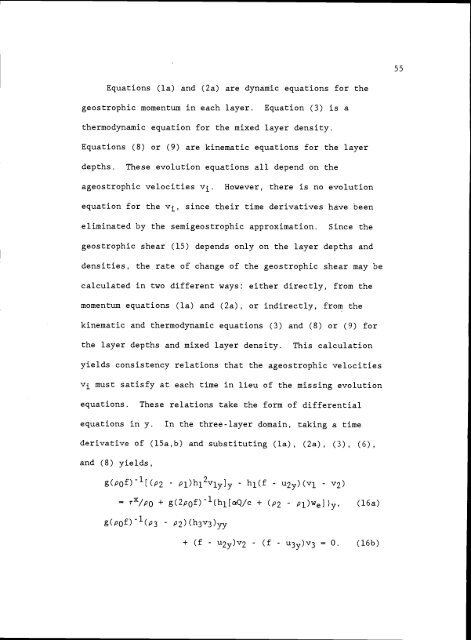
Equations (la) and (2a) are dynamic equations for the
geostrophic momentum in each layer. Equation (3) is a
thermodynamic equation for the mixed layer density.
Equations (8) or (9) are kinematic equations for the layer
depths. These evolution equations all depend on the
ageostrophic velocities vj. However, there is no evolution
equation for the v, since their time derivatives have been
eliminated by the semigeostrophic approximation. Since the
geostrophic shear (15) depends only on the layer depths and
densities, the rate of change of the geostrophic shear may be
calculated in two different ways: either directly, from the
momentum equations (la) and (2a), or indirectly, from the
kinematic and thermodynamic equations (3) and (8) or (9) for
the layer depths and mixed layer density. This calculation
yields consistency relations that the ageostrophic velocities
v must satisfy at each time in lieu of the missing evolution
equations. These relations take the form of differential
equations in y. In the three-layer domain, taking a time
derivative of (l5a,b) and substituting (la), (2a), (3), (6),
and (8) yields,
g(p0f)[(p2 Pl)hl2hllyly h1(f u2y)(Vl - v2)
TX/p0 + g(2p0fY-{h1[czQ/c + (P2 Pl)we])y, (l6a)
g(pof)(p3 - p2)(h3v3)
+ (f u2y)v2 - (f u3y)v3 = 0. (16b)
55