Observations and Modelling of Fronts and Frontogenesis

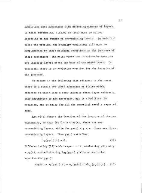
subdivided into subdomains with differing numbers of layers.
In these subdomains, (16a,b) or (16c) must be solved
according to the number of nonvanishing layers. In order to
close the problem, the boundary conditions (17) must be
supplemented by three matching conditions at the juncture of
these subdomains, the point where the interface between the
two interior layers meets the base of the mixed layer. In
addition, there is an evolution equation for the location of
the juncture.
We assume in the following that adjacent to the coast
there is a single two-layer subdomain of finite width,
offshore of which lies a semi-infinite three-layer subdomain.
This assumption is not necessary, but it simplifies the
notation, and it holds for all the numerical results reported
here.
Let y2(t) denote the location of the juncture of the two
subdomains, so that for 0 < y < y2(t), there are two
nonvariishing layers, while for y(t) < y < ,
nonvanishing layers. Then y2(t) satisfies,
there
are three
h2[y2(t),tJ = 0. (18)
Differentiating (18) with respect to t, evaluating (8b) at y
y2(t), and eliminating h(y,t) yields an evolution
equation for y2(t):
dy2/dt = v2[y2(t),t} + we[y2(t),tJ/h2y[y2(t),t}. (19)
57