Observations and Modelling of Fronts and Frontogenesis

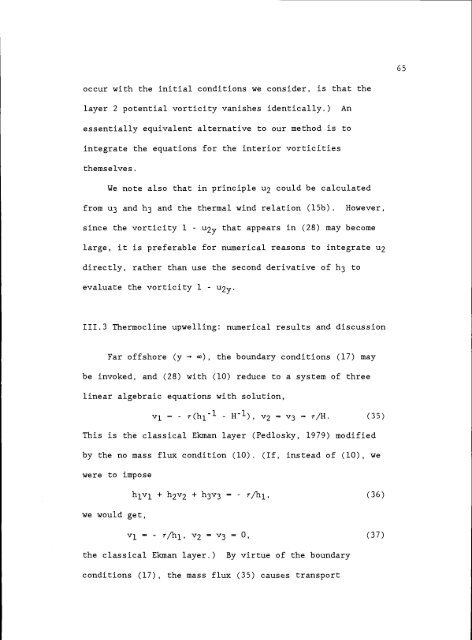
occur with the initial conditions we consider, is that the
layer 2 potential vorticity vanishes identically.) An
essentially equivalent alternative to our method is to
integrate the equations for the interior vorticities
themselves.
We note also that in principle u2 could be calculated
from u3 and h3 and the thermal wind relation (15b). However,
since the vorticity 1 U2y that appears in (28) may become
large, it is preferable for numerical reasons to integrate u2
directly, rather than use the second derivative of h3 to
evaluate the vorticity 1 U2y.
111.3 Thermocline upwelling: numerical results and discussion
Far offshore (y co), the boundary conditions (17) may
be invoked, and (28) with (10) reduce to a system of three
linear algebraic equations with solution,
V1 = - r(h1 - 111), v2 = = r/H. (35)
This is the classical Ekman layer (Pedlosky, 1979) modified
by the no mass flux condition (10). (If, instead of (10), we
were to impose
we would get,
h1v1 + h2v2 + h3v3 r/h1, (36)
v1 - r/h1, v2 = v3 = 0, (37)
the classical Ekman layer.) 3y virtue of the boundary
conditions (17), the mass flux (35) causes transport
65