Observations and Modelling of Fronts and Frontogenesis

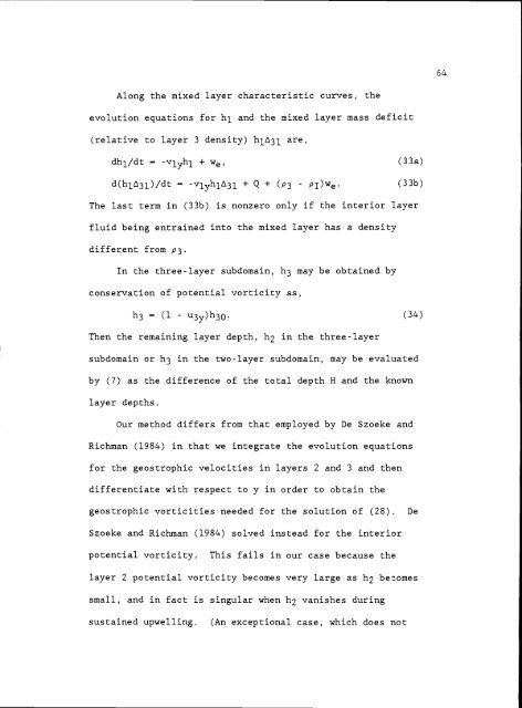
Along the mixed layer characteristic curves, the
evolution equations for h1 and the mixed layer mass deficit
(relative to layer 3 density) h131 are,
dh1/dt - vlyhl + We,
(33a)
d(h1i31)/dt = -vlyhlL3l Q + (P3 PI)We. (33b)
The last term in (33b) is nonzero only if the interior layer
fluid being entrained into the mixed layer has a density
different from p.
In the three-layer subdomain, h3 may be obtained by
conservation of potential vorticity as,
(1 u3y)h3o. (34)
Then the remaining layer depth, h2 in the three-layer
subdomain or h3 in the two-layer subdomain, may be evaluated
by (7) as the difference of the total depth H and the known
layer depths.
Our method differs from that employed by De Szoeke and
Richman (1984) in that we integrate the evolution equations
for the geostrophic velocities in layers 2 and 3 and then
differentiate with respect to y in order to obtain the
geostrophic vorticities needed for the solution of (28). De
Szoeke and Richman (1984) solved instead for the interior
potential vorticity. This fails in our case because the
layer 2 potential vorticity becomes very large as h2 becomes
small, and in fact is singular when h2 vanishes during
sustained upwelling. (An exceptional case, which does not
64