Observations and Modelling of Fronts and Frontogenesis

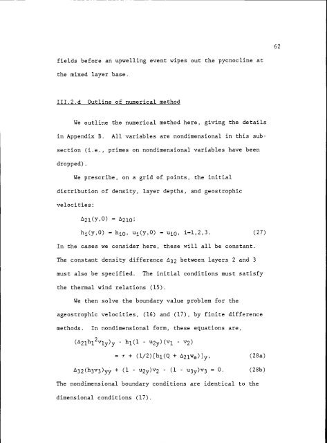
fields before an upwelling event wipes out the pycnocline at
the mixed layer base.
III.2.d Outline of numerical method
We outline the numerical method here, giving the details
in Appendix B. All variables are nondimensional in this sub-
section (i.e. , primes on nondimensional variables have been
dropped).
We prescribe, on a grid of points, the initial
distribution of density, layer depths, and geostrophic
velocities:
2l(Y,0) 2lo;
h(y,O) = ho, Ui(Y,O) uiO, i=l,2,3. (27)
In the cases we consider here, these will all be constant.
The constant density difference 32
between layers 2 and 3
must also be specified. The initial conditions must satisfy
the thermal wind relations (15).
We then solve the boundary value problem for the
ageostrophic velocities, (16) and (17), by finite difference
methods. In nondimensional form, these equations are,
(2l11l27ly)y h1(l u2y)(vl - v2)
= r + (l/2)[h1(Q + 2lWe)Jy (28a)
32th3hT3)yy + (1 u2y)v2 - (1 u3y)v3 = 0. (28b)
The nondimensional boundary conditions are identical to the
dimensional conditions (17).
62