- Page 1 and 2: Automated Aerial Image Analysis usi
- Page 3 and 4: Contents ii Page Certificate of Aut
- Page 5 and 6: List of Figures iv Page Figure 1: A
- Page 7 and 8: Abstract This study sets out an alg
- Page 9 and 10: The process was designed so that it
- Page 11 and 12: • Something capable of handling i
- Page 13 and 14: of a control to calibrate most of t
- Page 15 and 16: 1.2 General Introduction and Backgr
- Page 17 and 18: the higher the chances of successfu
- Page 19 and 20: overlaid aerial imagery. This is du
- Page 21 and 22: upper case, beginning with lower ca
- Page 23 and 24: a selected study area. This is poss
- Page 25 and 26: 2 Stepping through the Algorithm Th
- Page 27 and 28: The process can also be coded into
- Page 29 and 30: Aerial imagery is a form of databas
- Page 31 and 32: The software required for this step
- Page 33 and 34: study area from the photography and
- Page 35 and 36: The areas extracted were placed int
- Page 37 and 38: ands was detected the standard devi
- Page 39 and 40: 2.4 Confirmation The final stage of
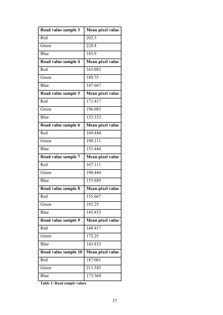
- Page 41 and 42: 3 Sampling for the Baseline Image K
- Page 43: Figure 3: Road area and vector data
- Page 47 and 48: Road test sample 2 Mean pixel value
- Page 49 and 50: 3.2 Water Figure 4: Typical Water A
- Page 51 and 52: The purpose of this thesis is to id
- Page 53 and 54: present in the target area (or its
- Page 55 and 56: possible to quickly process each se
- Page 57 and 58: Marsh Sample 1 Mean Pixel Value Sta
- Page 59 and 60: Marsh test Sample 1 (Pasture) Mean
- Page 61 and 62: form both pasture and road/ paving
- Page 63 and 64: Forest Sample 1 Mean pixel value St
- Page 65 and 66: Coniferous forestry test sample 1 (
- Page 67 and 68: whole was not analyzed but individu
- Page 69 and 70: infrared signatures to identify the
- Page 71 and 72: sampled in this study. In relation
- Page 73 and 74: 3.6 Track Figure 9: Typical Track A
- Page 75 and 76: surface area that might have been i
- Page 77 and 78: (Phynn et al, 2002). In this study
- Page 79 and 80: 3.7 Shade Figure 10: Typical Shade
- Page 81 and 82: currently available for all areas a
- Page 83 and 84: trends of bordering polygons mentio
- Page 85 and 86: 3.8 Roof Areas Figure 12: Typical R
- Page 87 and 88: Figure 13: Distribution of Building
- Page 89 and 90: These mean greyscale pixel values f
- Page 91 and 92: Roof test sample 1 Mean pixel value
- Page 93 and 94: 3.9 Pasture Figure 15: Typical Past
- Page 95 and 96:
From the above samples, samples 4 a
- Page 97 and 98:
For the track/ hard cover the diffe
- Page 99 and 100:
3.10 Rough Pasture Figure 16: Typic
- Page 101 and 102:
The identification of rough pasture
- Page 103 and 104:
cycle being suggested here to prese
- Page 105 and 106:
4 Testing This chapter describes a
- Page 107 and 108:
Figure 17: Creating the ASCII file
- Page 109 and 110:
Figure 20: Green colour band for pa
- Page 111 and 112:
Figure 23: Green colour band for pa
- Page 113 and 114:
The peak for the green colour band,
- Page 115 and 116:
Figure 30: Green colour band for pa
- Page 117 and 118:
Figure 31: Vector data for rough pa
- Page 119 and 120:
Figure 34: Green colour band for ro
- Page 121 and 122:
Figure 37: Green colour band for ro
- Page 123 and 124:
The peak for the green colour band,
- Page 125 and 126:
Figure 44: Green colour band for ro
- Page 127 and 128:
The first sample area came from a p
- Page 129 and 130:
Figure 47: Red colour band for mars
- Page 131 and 132:
Figure 50: Aerial view of marsh tes
- Page 133 and 134:
from which any variance would flag
- Page 135 and 136:
Figure 55: Red colour band for mars
- Page 137 and 138:
Figure 57: Aerial view of marsh tes
- Page 139 and 140:
4.4 Bog Test The sampling for areas
- Page 141 and 142:
Figure 62: Red colour band for bog
- Page 143 and 144:
Figure 65: Vector data for bog test
- Page 145 and 146:
The histogram for the green colour
- Page 147 and 148:
Figure 70: Aerial view for bog test
- Page 149 and 150:
This trend was continued for the bl
- Page 151 and 152:
The green colour band pixel count a
- Page 153 and 154:
4.5 Conclusion Image segmentation i
- Page 155 and 156:
5 Literature Review The goal of thi
- Page 157 and 158:
shown give a more detailed picture
- Page 159 and 160:
dependencies” (Kettling, P.330).
- Page 161 and 162:
identifying coffee plantations from
- Page 163 and 164:
apply an algorithm to colour the da
- Page 165 and 166:
In 2002 S. Phinn, M. Stanford, P. S
- Page 167 and 168:
with the authors work for a softwar
- Page 169 and 170:
ased analysis, solely spectral base
- Page 171 and 172:
16*16 pixels as urban or nonurban.
- Page 173 and 174:
as roads and car parks are so simil
- Page 175 and 176:
H. van der Werff and F. van der Mee
- Page 177:
Shen, S. S., Badhwar, G. D., and Ca