View/Open - ARAN

More documents

Recommendations

Info

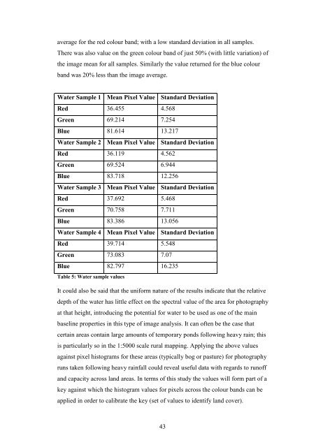
average for the red colour band; with a low standard deviation in all samples. There was also value on the green colour band of just 50% (with little variation) of the image mean for all samples. Similarly the value returned for the blue colour band was 20% less than the image average. Water Sample 1 Mean Pixel Value Standard Deviation Red 36.455 4.568 Green 69.214 7.254 Blue 81.614 13.217 Water Sample 2 Mean Pixel Value Standard Deviation Red 36.119 4.562 Green 69.524 6.944 Blue 83.718 12.256 Water Sample 3 Mean Pixel Value Standard Deviation Red 37.692 5.468 Green 70.758 7.711 Blue 83.386 13.056 Water Sample 4 Mean Pixel Value Standard Deviation Red 39.714 5.548 Green 73.083 7.07 Blue 82.797 16.235 Table 5: Water sample values It could also be said that the uniform nature of the results indicate that the relative depth of the water has little effect on the spectral value of the area for photography at that height, introducing the potential for water to be used as one of the main baseline properties in this type of image analysis. It can often be the case that certain areas contain large amounts of temporary ponds following heavy rain; this is particularly so in the 1:5000 scale rural mapping. Applying the above values against pixel histograms for these areas (typically bog or pasture) for photography runs taken following heavy rainfall could reveal useful data with regards to runoff and capacity across land areas. In terms of this study the values will form part of a key against which the histogram values for pixels across the colour bands can be applied in order to calibrate the key (set of values to identify land cover). 43
The purpose of this thesis is to identify an automated process for image analysis using vector data alongside a spectral analysis. The ability to extract water areas, in particular lakes or ponds with a large concentration of pixels of similar values, and establish a baseline value to calibrate the image key by would allow the user to target specific areas across successive runs of photography. This could be completed automatically using GDAL extract and returning the results of a histogram analysis. In order to gain a visual impression of the location of the main water bodies in the sample image the green and blue colour bands were mapped into the red, allowing the definition between the (relatively) monotone water and the remainder of the image. Figure 5: Water Area Image Modification The next part of the study involved taking separate sample areas from around the image and comparing them to the spectral values associated with water. The 44
Page 1 and 2: Automated Aerial Image Analysis usi
Page 3 and 4: Contents ii Page Certificate of Aut
Page 5 and 6: List of Figures iv Page Figure 1: A
Page 7 and 8: Abstract This study sets out an alg
Page 9 and 10: The process was designed so that it
Page 11 and 12: • Something capable of handling i
Page 13 and 14: of a control to calibrate most of t
Page 15 and 16: 1.2 General Introduction and Backgr
Page 17 and 18: the higher the chances of successfu
Page 19 and 20: overlaid aerial imagery. This is du
Page 21 and 22: upper case, beginning with lower ca
Page 23 and 24: a selected study area. This is poss
Page 25 and 26: 2 Stepping through the Algorithm Th
Page 27 and 28: The process can also be coded into
Page 29 and 30: Aerial imagery is a form of databas
Page 31 and 32: The software required for this step
Page 33 and 34: study area from the photography and
Page 35 and 36: The areas extracted were placed int
Page 37 and 38: ands was detected the standard devi
Page 39 and 40: 2.4 Confirmation The final stage of
Page 41 and 42: 3 Sampling for the Baseline Image K
Page 43 and 44: Figure 3: Road area and vector data
Page 45 and 46: (The previous samples were compared
Page 47 and 48: Road test sample 2 Mean pixel value
Page 49: 3.2 Water Figure 4: Typical Water A
Page 53 and 54: present in the target area (or its
Page 55 and 56: possible to quickly process each se
Page 57 and 58: Marsh Sample 1 Mean Pixel Value Sta
Page 59 and 60: Marsh test Sample 1 (Pasture) Mean
Page 61 and 62: form both pasture and road/ paving
Page 63 and 64: Forest Sample 1 Mean pixel value St
Page 65 and 66: Coniferous forestry test sample 1 (
Page 67 and 68: whole was not analyzed but individu
Page 69 and 70: infrared signatures to identify the
Page 71 and 72: sampled in this study. In relation
Page 73 and 74: 3.6 Track Figure 9: Typical Track A
Page 75 and 76: surface area that might have been i
Page 77 and 78: (Phynn et al, 2002). In this study
Page 79 and 80: 3.7 Shade Figure 10: Typical Shade
Page 81 and 82: currently available for all areas a
Page 83 and 84: trends of bordering polygons mentio
Page 85 and 86: 3.8 Roof Areas Figure 12: Typical R
Page 87 and 88: Figure 13: Distribution of Building
Page 89 and 90: These mean greyscale pixel values f
Page 91 and 92: Roof test sample 1 Mean pixel value
Page 93 and 94: 3.9 Pasture Figure 15: Typical Past
Page 95 and 96: From the above samples, samples 4 a
Page 97 and 98: For the track/ hard cover the diffe
Page 99 and 100: 3.10 Rough Pasture Figure 16: Typic
Page 101 and 102:
The identification of rough pasture
Page 103 and 104:
cycle being suggested here to prese
Page 105 and 106:
4 Testing This chapter describes a
Page 107 and 108:
Figure 17: Creating the ASCII file
Page 109 and 110:
Figure 20: Green colour band for pa
Page 111 and 112:
Page 113 and 114:
The peak for the green colour band,
Page 115 and 116:
Page 117 and 118:
Figure 31: Vector data for rough pa
Page 119 and 120:
Figure 34: Green colour band for ro
Page 121 and 122:
Page 123 and 124:
The peak for the green colour band,
Page 125 and 126:
Page 127 and 128:
The first sample area came from a p
Page 129 and 130:
Figure 47: Red colour band for mars
Page 131 and 132:
Figure 50: Aerial view of marsh tes
Page 133 and 134:
from which any variance would flag
Page 135 and 136:
Figure 55: Red colour band for mars
Page 137 and 138:
Figure 57: Aerial view of marsh tes
Page 139 and 140:
4.4 Bog Test The sampling for areas
Page 141 and 142:
Figure 62: Red colour band for bog
Page 143 and 144:
Figure 65: Vector data for bog test
Page 145 and 146:
The histogram for the green colour
Page 147 and 148:
Figure 70: Aerial view for bog test
Page 149 and 150:
This trend was continued for the bl
Page 151 and 152:
The green colour band pixel count a
Page 153 and 154:
4.5 Conclusion Image segmentation i
Page 155 and 156:
5 Literature Review The goal of thi
Page 157 and 158:
shown give a more detailed picture
Page 159 and 160:
dependencies” (Kettling, P.330).
Page 161 and 162:
identifying coffee plantations from
Page 163 and 164:
apply an algorithm to colour the da
Page 165 and 166:
In 2002 S. Phinn, M. Stanford, P. S
Page 167 and 168:
with the authors work for a softwar
Page 169 and 170:
ased analysis, solely spectral base
Page 171 and 172:
16*16 pixels as urban or nonurban.
Page 173 and 174:
as roads and car parks are so simil
Page 175 and 176:
H. van der Werff and F. van der Mee
Page 177:
Shen, S. S., Badhwar, G. D., and Ca
show all

View/Open - ARAN

You also want an ePaper? Increase the reach of your titles

Delete template?

Save as template?