Kinematic and Dynamic Analysis of Spatial Six Degree of Freedom ...

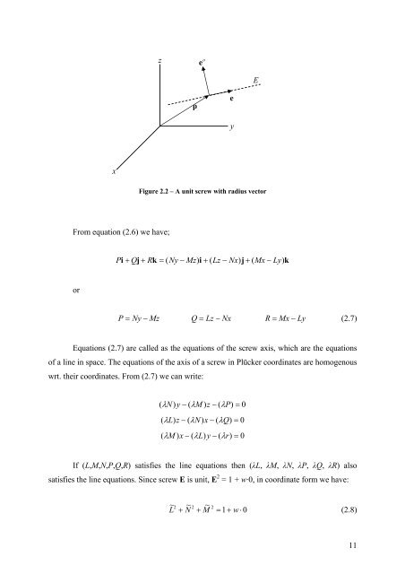
From equation (2.6) we have;
or
x
z
ρ
o
e
Figure 2.2 – A unit screw with radius vector
Pi + Qj
+ Rk
= ( Ny − Mz)
i + ( Lz − Nx)
j + ( Mx − Ly)
k
P = Ny − Mz Q = Lz − Nx R = Mx − Ly (2.7)
Equations (2.7) are called as the equations of the screw axis, which are the equations
of a line in space. The equations of the axis of a screw in Plücker coordinates are homogenous
wrt. their coordinates. From (2.7) we can write:
( λ N) y − ( λM
) z − ( λP)
= 0
( λ L) z − ( λN)
x − ( λQ)
= 0
( λ M ) x − ( λL)
y − ( λr)
= 0
If (L,M,N,P,Q,R) satisfies the line equations then (λL, λM, λN, λP, λQ, λR) also
satisfies the line equations. Since screw E is unit, E 2 = 1 + w·0, in coordinate form we have:
e
y
E
~ 2 ~ 2 ~ 2
L + N + M = 1+
w ⋅ 0
(2.8)
11