Kinematic and Dynamic Analysis of Spatial Six Degree of Freedom ...

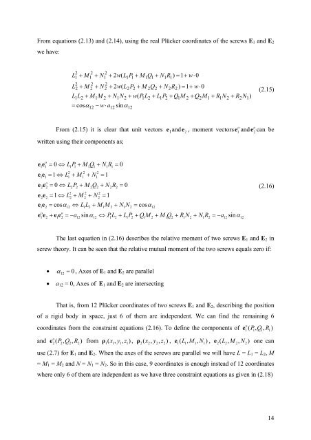
From equations (2.13) and (2.14), using the real Plücker coordinates of the screws E1 and E2
we have:
L
L
2
1
2
2
L L
1
+ M
+ M
2
2
1
2
2
+ M
12
+ N
+ N
1
M
2
1
2
2
2
= cosα
− w⋅
a
+ 2w(
L P + M Q + N R ) = 1+
w⋅
0
+ N
12
1
N
2
1
2
sinα
1
+ 2w(
L P + M Q
12
2
1
1
2
+ w(
P L
2
1
2
1
1
+ N
2
2
1
2
+ L P + Q M
From (2.15) it is clear that unit vectors e1and 2
written using their components as;
e e = 0 ⇔ L P + M Q + N R = 0
o
1 1
e e = 1 ⇔ L + M
1
o
2 2
2
1
o
1
1
e e
2
2
e e
2
o
1 2
2
1
12
1
= 1 ⇔ L
+ e e
2
2
2
1
2
12
2
1
+ M
2
2
1
1
2
2
1
+ N
e e = 0 ⇔ L P + M Q
12
2
1
2
+ N
2
2
1
1
= 1
+ N
2
= 1
2
1
1
R
2
2
= 0
e e = cosα
⇔ L L + M M + N N = cosα
1
1
2
2
1
12
2
1
R ) = 1+
w⋅
0
2
1
2
+ Q
2
M
1
+ R N
1
2
+ R
2
N
1
)
(2.15)
e , moment vectors o
e and o
e can be
= −a
sinα
⇔ PL
+ L P + Q M + M Q + R N + N R = −a
sinα
The last equation in (2.16) describes the relative moment of two screws E1 and E2 in
screw theory. It can be seen that the relative mutual moment of the two screws equals zero if:
• 12 0 = α , Axes of E1 and E2 are parallel
• a12 = 0, Axes of E1 and E2 are intersecting
That is, from 12 Plücker coordinates of two screws E1 and E2, describing the position
of a rigid body in space, just 6 of them are independent. We can find the remaining 6
o
coordinates from the constraint equations (2.16). To define the components of e P,
Q , R )
1
2
1
2
12
1
12
2
1 ( 1 1 1
o
and e P , Q , R ) from ρ x , y , z ) , ρ x , y , z ) , e L , M , N ) , e L , M , N ) one can
2(
2 2 2
1(
1 1 1
2(
2 2 2
1(
1 1 1
2(
2 2 2
(2.16)
use (2.7) for E1 and E2. When the axes of the screws are parallel we will have L = L1 = L2, M
= M1 = M2 and N = N1 = N2. So in this case, 9 coordinates is enough instead of 12 coordinates
where only 6 of them are independent as we have three constraint equations as given in (2.18)
14