Kinematic and Dynamic Analysis of Spatial Six Degree of Freedom ...

where
L
P
k
M
N
k
Q
R
k
k
k
k
=
=
=
=
=
−2
( Lj
D3
+ LiD2
± LijD1
) S αij
−2
( M jD3
+ M iD2
± M ijD1
) S αij
−2
( N jD3
+ NiD2
± NijD1
) S αij
o o o
−2
( ± PijD1
+ Pi
D2
+ Pj
D3
± LijD1
+ LiD2
+ L jD3
− Lk
f1)
S αij
o
o
o
−2
( ± QijD1
+ QiD2
+ Q jD3
± M ijD1
+ M iD2
+ M jD3
− M k f1)
S
o o
o
−2
( ± RijD1
+ RiD2
+ R jD3
± NijD1
+ NiD2
+ N jD3
− Nk
f1)
S αij
=
( ) 2 / 1
2
α − D Cα
− D C
D α
D = Cα
− Cα
Cα
1 = S ij 2 ki 3 jk
2 ki jk ij
D Cα
Cα
Cα
D Cα
Cα
Cα
3 = jk − ki ij
4 = ij − ki jk
−1
( D a Sα
+ D a Sα
+ D a Sα
)
o
D1 2 ki ki 3 jk jk 4 ij ij
= D
o
D2 = aij
Sαij
Cα
jk + a jk Sα
jk Cαij
− aki
Sαki
o
D3 = aij
Sαij
Cα
ki + aki
Sαki
Cαij
− a jk Sα
jk
ij = M iR
j − RiM
j + N jQi
Q j Ni
Qij = L j Ri
− R j Li
+ Ni
Pj
− Pi
N j
P −
R L Q − Q L + M P − P M
ij
= f aij
αij
2
1 = S
i
j
i
j
j
i
j
i
1
α
ij
(2.25)
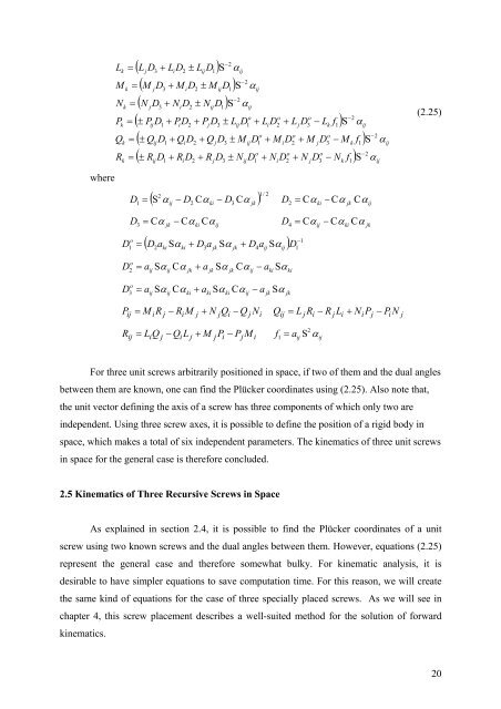
For three unit screws arbitrarily positioned in space, if two of them and the dual angles
between them are known, one can find the Plücker coordinates using (2.25). Also note that,
the unit vector defining the axis of a screw has three components of which only two are
independent. Using three screw axes, it is possible to define the position of a rigid body in
space, which makes a total of six independent parameters. The kinematics of three unit screws
in space for the general case is therefore concluded.
2.5 Kinematics of Three Recursive Screws in Space
As explained in section 2.4, it is possible to find the Plücker coordinates of a unit
screw using two known screws and the dual angles between them. However, equations (2.25)
represent the general case and therefore somewhat bulky. For kinematic analysis, it is
desirable to have simpler equations to save computation time. For this reason, we will create
the same kind of equations for the case of three specially placed screws. As we will see in
chapter 4, this screw placement describes a well-suited method for the solution of forward
kinematics.
20