Kinematic and Dynamic Analysis of Spatial Six Degree of Freedom ...

More documents

Recommendations

Info

( ( ( ) pc ( 2 s2 ) ) ) ( ) ( ) ( ( ) ) ( ) ( ) ( ) ( ) ( ) ( ( ) pc ( 3 s3 ) ) Fgn( u) := p c1, s1, r1, θ1, φ1, δ1− , , r1, θ3, φ3, δ3− Q Fgn( u) := Fgn( u) + p( c2, s2, r1, θ3, φ3, δ3) − pc ( 3, s3, r1, θ5, φ5, δ5) Fgn( u) := Fgn( u) + p( c1, s1, r1, θ1, φ1, δ1) − pc ( 3, s3, r1, θ5, φ5, δ5) Fgn( u) := Fgn( u) + p( c1, s1, r1, θ1, φ1, δ1) − pc ( 1, s1, r2, θ2, φ2, δ2) Fgn( u) := Fgn( u) + p( c2, s2, r1, θ3, φ3, δ3) − pc ( 2, s2, r2, θ4, φ4, δ4) Fgn( u) := Fgn( u) + p( c3, s3, r1, θ5, φ5, δ5) − pc ( 3, s3, r2, θ6, φ6, δ6) Fgn( u) := Fgn( u) + p( c1, s1, r2, θ2, φ2, δ2) − pc ( 2, s2, r2, θ4, φ4, δ4) Fgn( u) := Fgn( u) + p( c1, s1, r2, θ2, φ2, δ2) − pc ( 3, s3, r2, θ6, φ6, δ6) Fgn( u) := Fgn( u) + p( c3, s3, r2, θ6, φ6, δ6) − pc ( 2, s2, r2, θ4, φ4, δ4) Fgn( u) := Fgn( u) + p( c3, s3, r2, θ6, φ6, δ6) − pc ( 1, s1, r1, θ1, φ1, δ1) Fgn( u) := Fgn( u) + p( c1, s1, r2, θ2, φ2, δ2) − pc ( 2, s2, r1, θ3, φ3, δ3) − Q − Q − B − B − B − C − C − C − D − D Fgn( u) := Fgn( u) + p c2, s2, r2, θ4, φ4, δ4− , , r1, θ5, φ5, δ5− D u := ⎛ ⎜ ⎜ ⎜ ⎜ ⎜ ⎜ ⎜ ⎜ ⎜ ⎜ ⎜ ⎜ ⎜ ⎜ ⎜ ⎜ ⎜ ⎝ θ 2 θ 4 θ 6 φ 1 φ 2 φ 3 φ 4 φ 5 φ 6 δ 1 δ 3 δ 5 Soln T = ⎞ ⎟ ⎟ ⎟ ⎟ ⎟ ⎟ ⎟ ⎟ ⎟ ⎟ ⎟ ⎟ ⎟ ⎟ ⎟ ⎠ Kgn( u) := Fgn( u) Given u0 > 0.1 u6 > 0 u0 < π u6 < π u1 > 0.1 u7 > 0 u1 < π u7 < π u2 > 0.1 u8 > 0 u2 < π u8 < π Soln := Minimize( Kgn, u) u3 > 0 u9 > 0 u3 < π u9 < 2 u4 > 0 u10 > 0 u4 < π u10 < 2 Call routine u5 > 0 u11 > 0 u5 < π u11 < 2 84
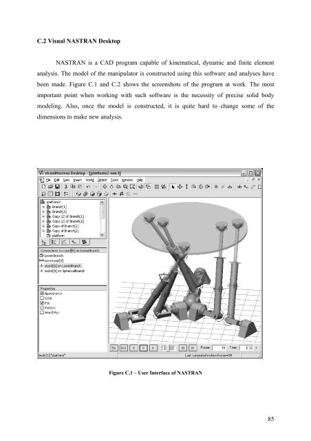
C.2 Visual NASTRAN Desktop NASTRAN is a CAD program capable of kinematical, dynamic and finite element analysis. The model of the manipulator is constructed using this software and analyses have been made. Figure C.1 and C.2 shows the screenshots of the program at work. The most important point when working with such software is the necessity of precise solid body modeling. Also, once the model is constructed, it is quite hard to change some of the dimensions to make new analysis. Figure C.1 – User Interface of NASTRAN 85
Page 1 and 2:
Kinematic and Dynamic Analysis of S
Page 3 and 4:
Research is what I'm doing when I d
Page 5 and 6:
ÖZ Bu tez yeni bir tip uzaysal alt
Page 7 and 8:
Chapter 4 KINEMATIC ANALYSIS ......
Page 9 and 10:
Figure 4.15 - Comparison of results
Page 11 and 12:
Chapter 1 INTRODUCTION The introduc
Page 13 and 14:
Figure 1.4 - The first flight simul
Page 15 and 16:
Generally, the actuators of a seria
Page 17 and 18:
−1 where J = J q J x . . . q = J
Page 19 and 20:
Chapter 2 SCREW KINEMATICS In this
Page 21 and 22:
From equation (2.6) we have; or x z
Page 23 and 24:
Using (2.7) and (2.12), one can fin
Page 25 and 26:
LP + MQ + NR = 0 L 1 2 2 + M 2 1 LP
Page 27 and 28:
Following Crammer’s method, the u
Page 29 and 30:
That’s, the variable angle α ki
Page 31 and 32:
~ ~ ~ ~ ~ ~ Let Ei ( Li , M i, Ni )
Page 33 and 34:
Qk = (NiPj + LjRi - LiRj - NjPi - a
Page 35 and 36:
The methods reported by F. Freudens
Page 37 and 38:
Using equations (3.4) and (3.6), we
Page 39 and 40:
Order of a structural group is the
Page 41 and 42:
3.3 Geometrical Structural Synthesi
Page 43 and 44: 3.4 Kinematic Structural Synthesis
Page 45 and 46: Let’s consider a 5 DOF parallel m
Page 47 and 48: Chapter 4 KINEMATIC ANALYSIS Kinema
Page 49 and 50: Figure 4.1 - The six degree of free
Page 51 and 52: v v v P4 = yv N 4 − zv M 4 v v v
Page 53 and 54: The best way of visualizing the dis
Page 55 and 56: 4.2.2 Results for the Actuation of
Page 63 and 64: Figure 4.17 - Corresponding piston
Page 65 and 66: Chapter 5 DYNAMIC ANALYSIS Dynamics
Page 67 and 68: Thus, according to Lagrange, the re
Page 69 and 70: J is the 6x6 Jacobian matrix that
Page 71 and 72: Chapter 6 DISCUSSION AND CONCLUSION
Page 73 and 74: REFERENCES [1] D. Stewart, A platfo
Page 75 and 76: [19] Seung-Bok Choi, Dong-Won Park,
Page 77 and 78: [38] Kotelnikov A. P., Screw calcul
Page 79 and 80: [60] R. I. Alizade, Investigation o
Page 81 and 82: A.1.1 CASSoM Source Code Like all v
Page 83 and 84: in the 'Input Parameters' section.
Page 85 and 86: pty:=roy+dy; ptz:=roz+dz; end; func
Page 87 and 88: Figure A.2 - a Screenshot of iMIDAS
Page 89 and 90: APPENDIX B RECURSIVE SYMBOLIC CALCU
Page 91 and 92: PP := L1 ← 0 M1 ← 0 N1 ← 1 L2
Page 93: Preleminary function definitions In
show all

Kinematic and Dynamic Analysis of Spatial Six Degree of Freedom ...

Create successful ePaper yourself

Delete template?

Save as template?