Kinematic and Dynamic Analysis of Spatial Six Degree of Freedom ...
Kinematic and Dynamic Analysis of Spatial Six Degree of Freedom ...
Kinematic and Dynamic Analysis of Spatial Six Degree of Freedom ...

Create successful ePaper yourself
Turn your PDF publications into a flip-book with our unique Google optimized e-Paper software.
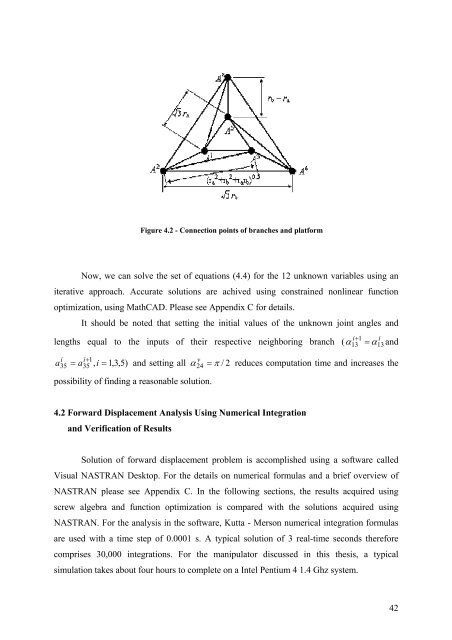
Figure 4.2 - Connection points <strong>of</strong> branches <strong>and</strong> platform<br />
Now, we can solve the set <strong>of</strong> equations (4.4) for the 12 unknown variables using an<br />
iterative approach. Accurate solutions are achived using constrained nonlinear function<br />
optimization, using MathCAD. Please see Appendix C for details.<br />
It should be noted that setting the initial values <strong>of</strong> the unknown joint angles <strong>and</strong><br />
lengths equal to the inputs <strong>of</strong> their respective neighboring branch ( α = α <strong>and</strong><br />
a<br />
i<br />
35<br />
i+<br />
1<br />
v<br />
= a , i = 1,<br />
3,<br />
5)<br />
<strong>and</strong> setting all α = π / 2 reduces computation time <strong>and</strong> increases the<br />
35<br />
possibility <strong>of</strong> finding a reasonable solution.<br />
4.2 Forward Displacement <strong>Analysis</strong> Using Numerical Integration<br />
<strong>and</strong> Verification <strong>of</strong> Results<br />
24<br />
Solution <strong>of</strong> forward displacement problem is accomplished using a s<strong>of</strong>tware called<br />
Visual NASTRAN Desktop. For the details on numerical formulas <strong>and</strong> a brief overview <strong>of</strong><br />
NASTRAN please see Appendix C. In the following sections, the results acquired using<br />
screw algebra <strong>and</strong> function optimization is compared with the solutions acquired using<br />
NASTRAN. For the analysis in the s<strong>of</strong>tware, Kutta - Merson numerical integration formulas<br />
are used with a time step <strong>of</strong> 0.0001 s. A typical solution <strong>of</strong> 3 real-time seconds therefore<br />
comprises 30,000 integrations. For the manipulator discussed in this thesis, a typical<br />
simulation takes about four hours to complete on a Intel Pentium 4 1.4 Ghz system.<br />
i+<br />
1<br />
13<br />
i<br />
13<br />
42