Publishers version - DTU Orbit

Pel/Pel,max [-]
1
0.98
0.96
0.94
0.92
0.9
−15 −10 −5 0 5 10 15
αH [deg]
Pel/Pel,max [-]
1
0.98
0.96
0.94
0.92
0.9
0 2 4 6 8 10 12 14 16
σ(αH) [deg]
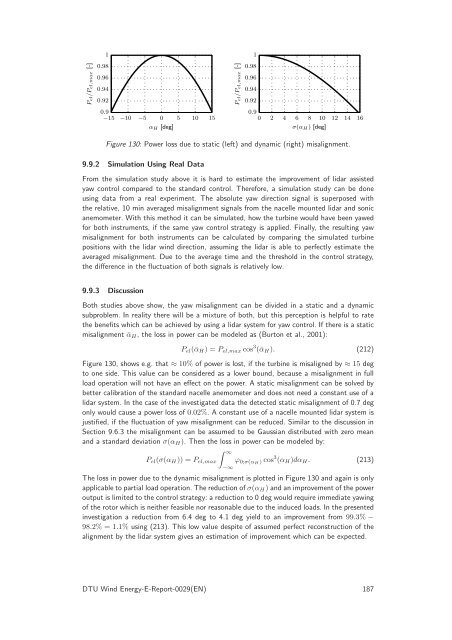
Figure 130: Power loss due to static (left) and dynamic (right) misalignment.
9.9.2 Simulation Using Real Data
From the simulation study above it is hard to estimate the improvement of lidar assisted
yaw control compared to the standard control. Therefore, a simulation study can be done
using data from a real experiment. The absolute yaw direction signal is superposed with
the relative, 10 min averaged misalignment signals from the nacelle mounted lidar and sonic
anemometer. With this method it can be simulated, how the turbine would have been yawed
for both instruments, if the same yaw control strategy is applied. Finally, the resulting yaw
misalignment for both instruments can be calculated by comparing the simulated turbine
positions with the lidar wind direction, assuming the lidar is able to perfectly estimate the
averaged misalignment. Due to the average time and the threshold in the control strategy,
the difference in the fluctuation of both signals is relatively low.
9.9.3 Discussion
Both studies above show, the yaw misalignment can be divided in a static and a dynamic
subproblem. In reality there will be a mixture of both, but this perception is helpful to rate
the benefits which can be achieved by using a lidar system for yaw control. If there is a static
misalignment ¯αH, the loss in power can be modeled as (Burton et al., 2001):
Pel(¯αH) = Pel,maxcos 3 (¯αH). (212)
Figure 130, shows e.g. that ≈ 10% of power is lost, if the turbine is misaligned by ≈ 15 deg
to one side. This value can be considered as a lower bound, because a misalignment in full
load operation will not have an effect on the power. A static misalignment can be solved by
better calibration of the standard nacelle anemometer and does not need a constant use of a
lidar system. In the case of the investigated data the detected static misalignment of 0.7 deg
only would cause a power loss of 0.02%. A constant use of a nacelle mounted lidar system is
justified, if the fluctuation of yaw misalignment can be reduced. Similar to the discussion in
Section 9.6.3 the misalignment can be assumed to be Gaussian distributed with zero mean
and a standard deviation σ(αH). Then the loss in power can be modeled by:
Pel(σ(αH)) = Pel,max
∞
−∞
ϕ 0;σ(αH)cos 3 (αH)dαH. (213)
The loss in power due to the dynamic misalignment is plotted in Figure 130 and again is only
applicabletopartialloadoperation.Thereductionofσ(αH) andanimprovementofthepower
output is limited to the control strategy: a reduction to 0 deg would require immediate yawing
of the rotor which is neither feasible nor reasonable due to the induced loads. In the presented
investigation a reduction from 6.4 deg to 4.1 deg yield to an improvement from 99.3% −
98.2% = 1.1% using (213). This low value despite of assumed perfect reconstruction of the
alignment by the lidar system gives an estimation of improvement which can be expected.
DTU Wind Energy-E-Report-0029(EN) 187