Publishers version - DTU Orbit

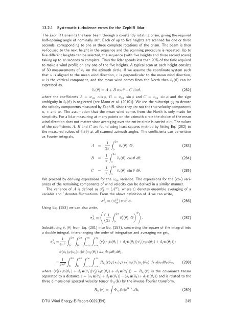
13.2.1 Systematic turbulence errors for the ZephIR lidar
The ZephIR transmits the laser beam through a constantly rotating prism, giving the required
half-opening angle of nominally 30 ◦ . Each of up to five heights are scanned for one or three
seconds, corresponding to one or three complete rotations of the prism. The beam is then
re-focused to the next height in the sequence and the scanning procedure is repeated. Up to
five different heights can be selected, the sequence (with five heights and three second scans)
taking up to 18 secondsto complete. Thus the lidar spends less than 20% of the time required
to make a wind profile on any one of the five heights. A typical scan at each height consists
of 50 measurements of vr on the azimuth circle. If we assume the coordinate system such
that u is aligned to the mean wind direction, v is perpendicular to the mean wind direction,
w is the vertical component, and the mean wind comes from the North then ˜vr(θ) can be
expressed as,
˜vr(θ) = A+Bcosθ+Csinθ, (282)
where the coefficients A = wqq cosφ, B = uqq sinφ and C = vqq sinφ and the sign
ambiguity in ˜vr(θ) is neglected (see Mann et al. (2010)). We use the subscript qq to denote
the velocitycomponentsmeasured byZephIR,since theyare not the true velocitycomponents
u, v and w. The assumption that the mean wind comes from the North is only made for
simplicity. For a lidar measuring at many points on the azimuth circle the choice of the mean
wind direction does not matter since averaging over the entire circle is carried out. The values
of the coefficients A, B and C are found using least squares method by fitting Eq. (282) to
the measured values of ˜vr(θ) at all scanned azimuth angles. The coefficients can be written
as Fourier integrals,
2π
A = 1
˜vr(θ) dθ, (283)
2π 0
B = 1
2π
˜vr(θ) cosθ dθ, (284)
π 0
C = 1
2π
˜vr(θ) sinθ dθ. (285)
π 0
We proceed by deriving expressions for the wqq variance. The expressions for the (co-) variances
of the remaining components of wind velocity can be derived in a similar manner.
The variance of A is defined as σ2 A = 〈A′2 〉, where 〈〉 denotes ensemble averaging of a
variable and ′ denotes fluctuations. From the above definition of A we can write,
Using Eq. (283) we can also write,
σ 2 A =
σ 2 A
= 〈w′2
qq 〉cos2 φ. (286)
2π
1
˜v
2π 0
′ 2
r (θ) dθ
. (287)
Substituting ˜vr(θ) from Eq. (281) into Eq. (287), converting the square of the integral into
a double integral, interchanging the order of integration and averaging we get,
σ 2 A = 1
4π 2
2π
2π
∞ ∞
0
0
−∞
−∞
ϕ(s1)ϕ(s2)ni(θ1)nj(θ2) ds1ds2dθ1dθ2,
= 1
4π 2
2π
2π
∞ ∞
0
0
−∞
−∞
〈v ′ i(s1n(θ1)+dfn(θ1))v ′ j(s2n(θ2)+dfn(θ2))〉
Rij(r)ϕ(s1)ϕ(s2)ni(θ1)nj(θ2) ds1ds2dθ1dθ2, (288)
where 〈v ′ i (s1n(θ1) + dfn(θ1))v ′ j (s2n(θ2) + dfn(θ2))〉 = Rij(r) is the covariance tensor
separated by a distance r = (s1n(θ1)+dfn(θ1))−(s2n(θ2)+dfn(θ2)) and is related to the
three dimensional spectral velocity tensor Φij(k) by the inverse Fourier transform,
Rij(r) = Φij(k)e ik·r dk, (289)
DTU Wind Energy-E-Report-0029(EN) 245