Publishers version - DTU Orbit

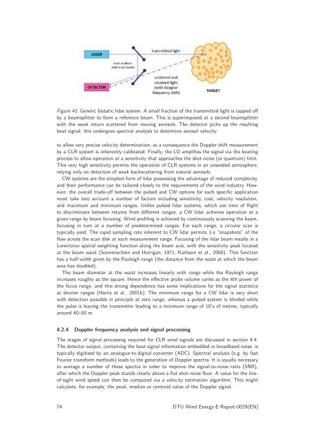
Figure 41: Generic bistatic lidar system. A small fraction of the transmitted light is tapped off
by a beamsplitter to form a reference beam. This is superimposed at a second beamsplitter
with the weak return scattered from moving aerosols. The detector picks up the resulting
beat signal; this undergoes spectral analysis to determine aerosol velocity.
to allow very precise velocity determination; as a consequence the Doppler shift measurement
by a CLR system is inherently calibrated. Finally, the LO amplifies the signal via the beating
process to allow operation at a sensitivity that approaches the shot-noise (or quantum) limit.
This very high sensitivity permits the operation of CLR systems in an unseeded atmosphere,
relying only on detection of weak backscattering from natural aerosols.
CW systems are the simplest form of lidar possessing the advantage of reduced complexity,
and their performance can be tailored closely to the requirements of the wind industry. However,
the overall trade-off between the pulsed and CW options for each specific application
must take into account a number of factors including sensitivity, cost, velocity resolution,
and maximum and minimum ranges. Unlike pulsed lidar systems, which use time of flight
to discriminate between returns from different ranges, a CW lidar achieves operation at a
given range by beam focusing. Wind profiling is achieved by continuously scanning the beam,
focusing in turn at a number of predetermined ranges. For each range, a circular scan is
typically used. The rapid sampling rate inherent to CW lidar permits 1-s “snapshots” of the
flow across the scan disk at each measurement range. Focusing of the lidar beam results in a
Lorentzian spatial weighting function along the beam axis, with the sensitivity peak located
at the beam waist (Sonnenschein and Horrigan, 1971; Karlsson et al., 2000). This function
has a half-width given by the Rayleigh range (the distance from the waist at which the beam
area has doubled).
The beam diameter at the waist increases linearly with range while the Rayleigh range
increases roughly as the square. Hence the effective probe volume varies as the 4th power of
the focus range, and this strong dependence has some implications for the signal statistics
at shorter ranges (Harris et al., 2001b). The minimum range for a CW lidar is very short
with detection possible in principle at zero range, whereas a pulsed system is blinded while
the pulse is leaving the transmitter leading to a minimum range of 10’s of metres, typically
around 40–50 m.
4.2.4 Doppler frequency analysis and signal processing
The stages of signal processing required for CLR wind signals are discussed in section 4.4.
The detector output, containing the beat signal information embedded in broadband noise, is
typically digitised by an analogue-to-digital converter (ADC). Spectral analysis (e.g. by fast
Fourier transform methods) leads to the generation of Doppler spectra. It is usually necessary
to average a number of these spectra in order to improve the signal-to-noise ratio (SNR),
after which the Doppler peak stands clearly above a flat shot-noise floor. A value for the lineof-sight
wind speed can then be computed via a velocity estimation algorithm. This might
calculate, for example, the peak, median or centroid value of the Doppler signal.
74 DTU Wind Energy-E-Report-0029(EN)