Dirac Fermions in Graphene and Graphite—a view from angle ...

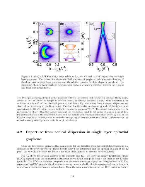
Figure 4.1. (a-c) ARPES intensity maps taken at E F , -0.4 eV and -1.2 eV respectively on single
layer graphene. The dotted line shows the Brillouin zone of graphene. (d) schematic drawing of
the dispersion in single layer graphene and the relative energies for data shown in panels a-c. (e)
Dispersion of single layer graphene measured along a high symmetric direction through the K point
(see black line in the inset).
The Dirac point energy, defined as the midpoint between the valence and conduction bands at the K point,
occurs at -0.4 eV since the sample is electron doped, as already discussed above. More importantly, in
addition to this shift of the chemical potential and hence E D , deviations from a conical dispersion are
observed in the vicinity of the Dirac point. The first, hardly visible on the energy scale of this figure, is at
approximately -0.2 eV below E F and is due to coupling to phonons 66,67,68 . The second occurs near E D . In
particular, we observe that the valence band and the conduction band do not merge at a single point at E D ,
but instead the top of the conduction bands and the bottom of the valence bands stop before E F and at the
K point there is an intensity over an extended energy region between these two bands. Understanding the
second anomaly near E D is the main focus of this chapter.
4.2 Departure from conical dispersion in single layer epitaxial
graphene
There are two possible scenarios that can account for the deviation from the conical dispersion near E D
discussed in the previous section. These include many body interaction and the opening of a gap at the K
point. As we will show below the latter is the most likely scenario to account for the anomaly.
Fig. 4.2 shows the detailed analysis of the anomaly near E D . We show the energy distribution curves
(EDCs) in panel c and the momentum distribution curves (MDCs) in panel d for a cut taken at the K point
(panel b). The EDCs show always two peaks with the minimum energy separation, being realized at K. The
presence of two EDC peaks in the all momentum range, even at the K point, is a strong evidence in favor of a
gap between the conduction and valence band. From the separation between the two EDC peaks we deduce
25