Dirac Fermions in Graphene and Graphiteâa view from angle ...

More documents

Recommendations

Info

Figure 7.6. ARPES intensity map measured on HOPG near the BZ corners at photon energies of 43 (k z ≈ 0.35 c ∗ ) and 55 eV (k z ≈ 0.10 c ∗ ) respectively. AB and BB label the antibonding and bonding π bands. (c-d) MDCs at -1.2 eV for data shown in panels a and b respectively. (e-f) ARPES intensity map measured on single crystal graphite near the zone corner at photon energies of 140 eV (k z ≈ 0.50 c ∗ ) and 80 eV (k z ≈ 0.07 c ∗ ) respectively. (g-h) MDCs at -1.2 eV for data shown in panels e and f. clearly distinguish three nondispersive features at -2.9 eV, -4.3 eV and -7.8 eV, indicated by arrows on the same figure. The nondispersive nature of the features can be checked by the EDCs shown in panels b and c. These features, appearing as sharp extended horizontal lines in panel a suggests the presence of nondispersive localized states. The energies of these nondispersive features occur at the top and bottom of the dispersive band and these features are strongly connected with the dispersive features associated with the π and σ bands. Thus we have associated the presence of such nondispersive features to the elastic scattering of electrons in either the initial state or the final state by inhomogeneity or disorder 101 . We now discuss the more important effect of disorder in the low energy electronic properties, as observed in all types of graphite samples. In order to investigate this effect, we have performed position dependent ARPES study with main focus on the near E F states. Each spectrum is averaged over ≈ 100 µm, the spot size of the synchrotron beam. We find that some of the low energy properties of the electronic structure are indeed strongly position dependent and we associate them with the presence of disordered states. We note that similar behavior has been observed in both single crystal graphite and HOPG, suggesting that these are important properties associated with these materials. In Fig. 7.8 we report typical ARPES intensity map near E F for an HOPG sample (panels a, b) and single crystal graphite (panel c, d), taken in different positions on the same sample. While panels a and c show a parabolic π band dispersion, it is clear that, as we change position on the sample (panels b, d) within the same sample we observe an additional weakly-dispersive electron-like feature, within 50 meV below E F (panels b, d), coexisting with the parabolic π band. Note that while the presence of the π band is position independent, observed in all the samples studied for all positions measured, this additional electron-like feature is strongly position dependent, for each of the sample studied. We now discuss the origin of this feature. While it seems appealing to associate this electron-like feature with the electron pocket predicted by band structure at k z =0, we note that its position dependence as well as the detailed analysis of the effective mass and carrier concentration (discussed in details later), clearly suggests a different origin for this feature. Fig. 7.9 shows the details of this additional band near E F , from data taken on HOPG. The details of this electron-like band and the π band are analyzed from the MDCs and EDCs shown in panels b-g. Panel b shows the MDC at E F . A main peak in the center, associated with the π band, and two side peaks associated with the additional band, can be distinguished. As the binding energy increases, the low energy band is no longer present and the peaks in the MDC at -100 meV (panel c) are from the main π band. However, the dispersions of the low energy bands are difficult to follow, partly due to the highly parabolic bands in this 57
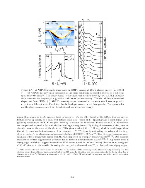
Figure 7.7. (a) ARPES intensity map taken on HOPG sample at 26 eV photon energy (k z ≈ 0.13 c ∗ ). (b) ARPES intensity map measured at the same conditions as panel a except on a different spot inside the sample. The arrow points to the additional intensity near E F . (c) ARPES intensity map measured on single crystal graphite with 50 eV photon energy. The dotted line is extracted dispersion from EDCs. (d) ARPES intensity maps measured at the same conditions as panel c except on a different spot. The dotted line is the dispersion extracted from panel c. The open circles are the dispersions extracted for the additional feature at low energy. region that makes an MDC analysis hard to interpret. On the other hand, in the EDCs, this low energy feature shows up clearly as a small well-defined peak at k 1 (panel e), k 12 (panel g) and a small hump in k 7 (panel f) and thus we use EDC analysis (panel d) to extract the dispersion. The extracted EDC dispersions are overplotted in panel a for both the low and high energy bands. By fitting the electron pocket, we can directly measure the mass of the electrons. This gives a value 0.42 ± 0.07 m e , which is much larger than that of electrons and holes as measured in transport 112,111,114 . Also, by estimating the volume of the large electron pocket 4 , we obtain an electron concentration of 8.0±0.7×10 19 cm −3 . This electron concentration is again an order of magnitude higher than the value reported by transport measurements 112,111 . One possible explanation for this large electron pocket is due to defect-induced localized states 116,83,129 , e.g. states along a zigzag edge. Additional support comes from STM, where a peak in the local density of states at an energy (≈ -0.03 eV) similar to the weakly dispersing electron pocket discussed here 115 , is observed near zigzag edges. 4 The concentration of electrons can be estimated by the volume of the electron pocket. This is done by assuming that the electron pocket is an ellipsoid that occupies half of the BZ along k z direction, and the cross section in the k x-k y plane has a diameter of ≈ 0.1Å −1 . This gives a volume of ≈ 1.2±0.1×10 −4 of the BZ size, which corresponds to the electron concentration here estimated. 58
Page 1 and 2:
Dirac Fermions in Graphene and Grap
Page 3 and 4:
Dirac Fermions in Graphene and Grap
Page 5 and 6:
Contents Abstract 1 Contents Acknow
Page 7 and 8:
7.6 Conclusions and implication of
Page 9 and 10:
Curriculum Vitæ Shuyun Zhou Educat
Page 11 and 12:
• Selected as Science Highlight f
Page 13 and 14:
The unit cell of graphene contains
Page 15 and 16:
Projecting this equation into φ(r
Page 17 and 18: Figure 1.5. Schematic drawing of th
Page 19 and 20: Chapter 2 Experimental techniques 2
Page 21 and 22: dispersion E(k z ). Thus k z values
Page 23 and 24: where ɛ is infinitely small. Accor
Page 25 and 26: Langmuirs (1L=10 −6 torr·s) to c
Page 27 and 28: mean free path, E kin is the kineti
Page 29 and 30: a b c d e f graphite SiC f graphite
Page 31 and 32: Figure 3.3. XPS results showing dat
Page 33 and 34: Figure 3.5. Intensity map at -1 eV
Page 35 and 36: Chapter 4 Gap opening in epitaxial
Page 37 and 38: Figure 4.2. Observation of the gap
Page 39 and 40: the EDCs as well as the region of e
Page 41 and 42: Figure 4.7. Dispersions measured in
Page 43 and 44: Figure 4.9. (a-c) LEEM images taken
Page 45 and 46: Figure 4.10. Proposed mechanism for
Page 47 and 48: Chapter 5 Metal-insulator transitio
Page 49 and 50: Figure 5.2. (a) Dispersions through
Page 51 and 52: Figure 5.3. (a-f) Data taken throug
Page 53 and 54: Chapter 6 Dirac fermions and effect
Page 55 and 56: Figure 6.2. Linear Λ-shaped disper
Page 57 and 58: Figure 6.4. Detailed low energy dis
Page 59 and 60: Figure 6.6. Detailed dispersion nea
Page 61 and 62: Chapter 7 ARPES study of partially
Page 63 and 64: Figure 7.2. (a) Fermi energy intens
Page 65 and 66: direction, i.e. perpendicular to gr
Page 67: Figure 7.5. ARPES intensity map mea
Page 71 and 72: Figure 7.9. (a) ARPES intensity map
Page 73 and 74: 19. Hüfner, S. Photoelectron Spect
Page 75 and 76: 59. Jiang, Y. J., Yao, D.-Y., Carls
Page 77 and 78: 99. Luk’yanchuk, I. A. & Kopelevi
Page 79 and 80: List of Figures 1.1 (a) Sp 2 bondin
Page 81 and 82: 4.8 Thickness dependence of E D and
Page 83 and 84: 7.2 (a) Fermi energy intensity map.
show all

Dirac Fermions in Graphene and Graphiteâa view from angle ...

You also want an ePaper? Increase the reach of your titles

Delete template?

Save as template?

Dirac Fermions in Graphene and Graphiteâa view from angle ...