Probabilistic Performance Analysis of Fault Diagnosis Schemes

More documents

Recommendations

Info

α β W 1 ∆ W 2 u v f (θ) G y . F r Figure 6.7. Block diagram of a linearized vertical take-off and landing (vtol) aircraft model with additive model uncertainty. 6.4 VTOL Aircraft Example In this section, we examine the effects of additive model uncertainty on the performance of an observer-based fault detection scheme. The system under consideration is is a linearized model of the longitudinal dynamics of a vertical take-off and landing (vtol) aircraft. The original modeling and linearization of this system are due to Narendra and Tripathi [70]. Since the publication of [70], variants of this model have been used in a number of fault detection studies (e.g., [83, 94–96, 102]). 6.4.1 Problem Formulation Consider the block diagram shown in Figure 6.7. The additive uncertainty affects the map from the input u to the output y. Assume that both W 1 and W 2 are fixed square matrices, and assume that ∆ ∈ ∆ 2,ltv (γ). The continuous-time dynamics of the system are of the form where the states and inputs are defined as ẋ = Ax + B u u + B v v + B f f (θ), y = C x + ( D u +W 2 ∆W 1 ) u + Dv v, ⎡ ⎤ horizontal velocity (knots) [ ] vertical velocity (knots) x = ⎢ ⎥ ⎣ pitch rate (deg/s) ⎦ , u = collective pitch control longitudinal pitch control pitch angle (deg) 109
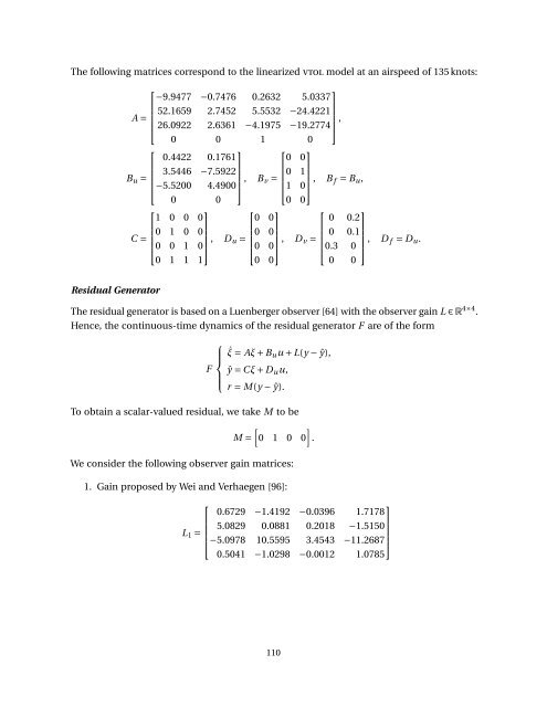
The following matrices correspond to the linearized vtol model at an airspeed of 135 knots: ⎡ ⎤ −9.9477 −0.7476 0.2632 5.0337 52.1659 2.7452 5.5532 −24.4221 A = ⎢ ⎥ ⎣ 26.0922 2.6361 −4.1975 −19.2774⎦ , 0 0 1 0 ⎡ ⎤ ⎡ ⎤ 0.4422 0.1761 0 0 3.5446 −7.5922 B u = ⎢ ⎥ ⎣−5.5200 4.4900⎦ , B 0 1 v = ⎢ ⎥ ⎣1 0⎦ , B f = B u , 0 0 0 0 ⎡ ⎤ ⎡ ⎤ ⎡ ⎤ 1 0 0 0 0 0 0 0.2 0 1 0 0 C = ⎢ ⎥ ⎣0 0 1 0⎦ , D 0 0 u = ⎢ ⎥ ⎣0 0⎦ , D 0 0.1 v = ⎢ ⎥ ⎣0.3 0 ⎦ , D f = D u . 0 1 1 1 0 0 0 0 Residual Generator The residual generator is based on a Luenberger observer [64] with the observer gain L ∈ R 4×4 . Hence, the continuous-time dynamics of the residual generator F are of the form ⎧ ⎪⎨ ˙ξ = Aξ + B u u + L(y − ŷ), F ŷ = Cξ + D u u, ⎪⎩ r = M(y − ŷ). To obtain a scalar-valued residual, we take M to be [ ] M = 0 1 0 0 . We consider the following observer gain matrices: 1. Gain proposed by Wei and Verhaegen [96]: ⎡ ⎤ 0.6729 −1.4192 −0.0396 1.7178 5.0829 0.0881 0.2018 −1.5150 L 1 = ⎢ ⎥ ⎣−5.0978 10.5595 3.4543 −11.2687⎦ 0.5041 −1.0298 −0.0012 1.0785 110
Page 1 and 2:
Probabilistic Performance Analysis
Page 3 and 4:
Abstract Probabilistic Performance
Page 5 and 6:
Soli Deo gloria. i
Page 7 and 8:
3 Probabilistic Performance Analysi
Page 9 and 10:
List of Figures 2.1 “Bathtub” s
Page 11 and 12:
List of Tables 4.1 Time-complexity
Page 13 and 14:
Acknowledgements When I started wri
Page 15 and 16:
tic metrics that rigorously quantif
Page 17 and 18:
tion. • Complexity of Markov Chai
Page 19 and 20:
Given an event B ∈ F with P(B) >
Page 21 and 22:
Note that E ( f (x) | y ) is a rand
Page 23 and 24:
for all c ∈ R, where erf(c) := 2
Page 25 and 26:
Hazard Rate λ 0 0 break-in 0 t 1 t
Page 27 and 28:
malfunction — an intermittent irr
Page 29 and 30:
where the matrix Q is chosen to app
Page 31 and 32:
v w u G θ y F r δ V d Figure 2.3.
Page 33 and 34:
These relationships can be used to
Page 35 and 36:
ε Residual 0 0 T f T d Time Figure
Page 37 and 38:
Chapter 3 Probabilistic Performance
Page 39 and 40:
the worst-case performance under a
Page 41 and 42:
For example, P tp,k = P(D 1,k ∩ H
Page 43 and 44:
where the subscript k has been omit
Page 45 and 46:
1 (α 3 ,β 3 ) Pd,k Probability of
Page 47 and 48:
Definition 3.9. The upper boundary
Page 49 and 50:
1 ε increasing ε = 0 Pd,k Probabi
Page 51 and 52:
1 P d,k P f,k β Q 0,k Probability
Page 53 and 54:
In general, as Q 0,k decreases, the
Page 55 and 56:
from J k by taking column-sums. If
Page 57 and 58:
Chapter 4 Computational Framework 4
Page 59 and 60:
Fact 4.1. Given a Markov chain θ
Page 61 and 62:
v 1 v 2 v 3 v 4 Figure 4.1. Simple
Page 63 and 64:
for some p ∈ (0,1). Then, the cor
Page 65 and 66:
Proof. Let ϑ 0:l be a possible pat
Page 67 and 68:
the matrix A as in Theorem 4.12. Th
Page 69 and 70:
every 1-bit of b i is a 1-bit of b
Page 71 and 72: Assumed Structure of the Residual G
Page 73 and 74: Therefore, conditional on the event
Page 75 and 76: In the non-scalar case (i.e., r k
Page 77 and 78: probability matrix is given by ( Λ
Page 79 and 80: s 2 . .. s 0 s 1 s q Figure 4.4. St
Page 81 and 82: metrics at time k are defined as Ĵ
Page 83 and 84: Proposition 4.32. Let N be the fina
Page 85 and 86: Algorithm 4.2. Procedure for comput
Page 87 and 88: Second, we show that the running ti
Page 89 and 90: Table 4.1. Time-complexity of compu
Page 91 and 92: For p ∈ [1,∞], the l p -norm ba
Page 93 and 94: linear time-varying uncertainties
Page 95 and 96: for the appropriate choice of k f a
Page 97 and 98: Hence, it is straightforward to sho
Page 99 and 100: v w f (θ) u G θ y . F r Figure 5.
Page 101 and 102: Maximizing the Probability of False
Page 103 and 104: β ∆ α v f (θ) u G θ y . F r F
Page 105 and 106: β ∆ α β ∆ 1 . .. ∆q α (a)
Page 107 and 108: if and only if [ T (βi ) T T (M i
Page 109 and 110: Fix a parameter sequence θ = ϑ an
Page 111 and 112: As in Section 5.2.2, if the matrix
Page 113 and 114: Chapter 6 Applications 6.1 Introduc
Page 115 and 116: p t p s v t + f t (θ) φ γ ˆV ĥ
Page 117 and 118: 300 18 V (m/s) 200 h (km) 12 Airspe
Page 119 and 120: 1 P tn,k 0.8 P fp,k P fn,k (a) Prob
Page 121: 0.4 Probability of False Alarm, P
Page 125 and 126: 6.4.2 Applying the Framework The ma
Page 127 and 128: P ⋆ f Probability of False Alarm,
Page 129 and 130: Chapter 7 Conclusions & Future Work
Page 131 and 132: measurement noise. Hence, the appli
Page 133 and 134: [12] R. H. Chen, D. L. Mingori, and
Page 135 and 136: [40] R. L. Graham, D. E. Knuth, and
Page 137 and 138: [68] L. A. Mironovski, Functional d
Page 139 and 140: [95] H. B. Wang, J. L. Wang, and J.
show all

Probabilistic Performance Analysis of Fault Diagnosis Schemes

You also want an ePaper? Increase the reach of your titles

Delete template?

Save as template?