Probabilistic Performance Analysis of Fault Diagnosis Schemes

More documents

Recommendations

Info

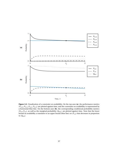
1 P tn,k a P fp,k P fn,k (a) Probability P tp,k 0 0 k f N 1 Time, k P d,k P f,k Q 0,k (b) Probability 0 0 k f N Time, k Figure 3.5. Visualization of a constraint on availability. On the top axes (a), the performance metrics {P tn,k ,P fp,k ,P fn,k ,P tp,k } are plotted against time, and the constraint on availability is represented by a horizontal blue line. On the bottom axes (b), the corresponding conditional probability metrics {P d,k ,P f,k }, as well as the marginal probability {Q 0,k }, are plotted against time. Note that the lower bound on availability a translates to an upper bound (blue line) on {P f,k } that decreases in proportion to {Q 0,k }. 37
1 P d,k P f,k β Q 0,k Probability α 0 0 N Time, k Figure 3.6. Visualization of a constraint on the performance metrics {P f,k } and {P d,k } over time. Here, the constraint is P d,k > β and P f,k < α, for k = 0,1,..., N . The marginal probability that the system is in the nominal mode, denoted {Q 0,k }, is shown for reference. steady-state performance metrics if k m is large enough. 3.5.2 Bound on Bayesian Risk As discussed in Section 3.3.3, the Bayesian risk provides a general linear framework for aggregating the performance of a fault detection scheme into a single performance metric. For the sake of simplicity, assume that the loss matrix L ∈ R 2 is constant for all time. Given a sequence { ¯R k }, such that ¯R k > 0 for all k, the bound on the Bayesian risk at time k is R k (Q,V ) = L 00 Q 0,k + L 01 Q 1,k + (L 01 − L 00 )P f,k Q 0,k + (L 11 − L 10 )P d,k Q 1,k < ¯R k . At each k, the set of performance points (P f,k ,P d,k ) satisfying this bound is the intersection of some half-space in R 2 with the roc space [0,1] 2 (see Figure 3.8). The boundary of this half-space is determined the loss matrix L and the probability Q 0,k . Clearly, if the ideal performance point (0,1) does not lie in this half-space at time k, then the bound R k < ¯R k is too stringent. Note that as Q 0,k → 1, the bound on risk approaches L 00 + (L 01 − L 00 )P f,k < ¯R ⇐⇒ P f,k < ¯R − L 00 L 01 − L 00 . Similarly, as Q 0,k → 0, the bound approaches L 01 + (L 11 − L 10 )P d,k < ¯R ⇐⇒ P d,k > L 01 − ¯R L 10 − L 11 . 38
Page 1 and 2: Probabilistic Performance Analysis
Page 3 and 4: Abstract Probabilistic Performance
Page 5 and 6: Soli Deo gloria. i
Page 7 and 8: 3 Probabilistic Performance Analysi
Page 9 and 10: List of Figures 2.1 “Bathtub” s
Page 11 and 12: List of Tables 4.1 Time-complexity
Page 13 and 14: Acknowledgements When I started wri
Page 15 and 16: tic metrics that rigorously quantif
Page 17 and 18: tion. • Complexity of Markov Chai
Page 19 and 20: Given an event B ∈ F with P(B) >
Page 21 and 22: Note that E ( f (x) | y ) is a rand
Page 23 and 24: for all c ∈ R, where erf(c) := 2
Page 25 and 26: Hazard Rate λ 0 0 break-in 0 t 1 t
Page 27 and 28: malfunction — an intermittent irr
Page 29 and 30: where the matrix Q is chosen to app
Page 31 and 32: v w u G θ y F r δ V d Figure 2.3.
Page 33 and 34: These relationships can be used to
Page 35 and 36: ε Residual 0 0 T f T d Time Figure
Page 37 and 38: Chapter 3 Probabilistic Performance
Page 39 and 40: the worst-case performance under a
Page 41 and 42: For example, P tp,k = P(D 1,k ∩ H
Page 43 and 44: where the subscript k has been omit
Page 45 and 46: 1 (α 3 ,β 3 ) Pd,k Probability of
Page 47 and 48: Definition 3.9. The upper boundary
Page 49: 1 ε increasing ε = 0 Pd,k Probabi
Page 53 and 54: In general, as Q 0,k decreases, the
Page 55 and 56: from J k by taking column-sums. If
Page 57 and 58: Chapter 4 Computational Framework 4
Page 59 and 60: Fact 4.1. Given a Markov chain θ
Page 61 and 62: v 1 v 2 v 3 v 4 Figure 4.1. Simple
Page 63 and 64: for some p ∈ (0,1). Then, the cor
Page 65 and 66: Proof. Let ϑ 0:l be a possible pat
Page 67 and 68: the matrix A as in Theorem 4.12. Th
Page 69 and 70: every 1-bit of b i is a 1-bit of b
Page 71 and 72: Assumed Structure of the Residual G
Page 73 and 74: Therefore, conditional on the event
Page 75 and 76: In the non-scalar case (i.e., r k
Page 77 and 78: probability matrix is given by ( Λ
Page 79 and 80: s 2 . .. s 0 s 1 s q Figure 4.4. St
Page 81 and 82: metrics at time k are defined as Ĵ
Page 83 and 84: Proposition 4.32. Let N be the fina
Page 85 and 86: Algorithm 4.2. Procedure for comput
Page 87 and 88: Second, we show that the running ti
Page 89 and 90: Table 4.1. Time-complexity of compu
Page 91 and 92: For p ∈ [1,∞], the l p -norm ba
Page 93 and 94: linear time-varying uncertainties
Page 95 and 96: for the appropriate choice of k f a
Page 97 and 98: Hence, it is straightforward to sho
Page 99 and 100: v w f (θ) u G θ y . F r Figure 5.
Page 101 and 102:
Maximizing the Probability of False
Page 103 and 104:
β ∆ α v f (θ) u G θ y . F r F
Page 105 and 106:
β ∆ α β ∆ 1 . .. ∆q α (a)
Page 107 and 108:
if and only if [ T (βi ) T T (M i
Page 109 and 110:
Fix a parameter sequence θ = ϑ an
Page 111 and 112:
As in Section 5.2.2, if the matrix
Page 113 and 114:
Chapter 6 Applications 6.1 Introduc
Page 115 and 116:
p t p s v t + f t (θ) φ γ ˆV ĥ
Page 117 and 118:
300 18 V (m/s) 200 h (km) 12 Airspe
Page 119 and 120:
1 P tn,k 0.8 P fp,k P fn,k (a) Prob
Page 121 and 122:
0.4 Probability of False Alarm, P
Page 123 and 124:
The following matrices correspond t
Page 125 and 126:
6.4.2 Applying the Framework The ma
Page 127 and 128:
P ⋆ f Probability of False Alarm,
Page 129 and 130:
Chapter 7 Conclusions & Future Work
Page 131 and 132:
measurement noise. Hence, the appli
Page 133 and 134:
[12] R. H. Chen, D. L. Mingori, and
Page 135 and 136:
[40] R. L. Graham, D. E. Knuth, and
Page 137 and 138:
[68] L. A. Mironovski, Functional d
Page 139 and 140:
[95] H. B. Wang, J. L. Wang, and J.
show all

Probabilistic Performance Analysis of Fault Diagnosis Schemes

Create successful ePaper yourself

Delete template?

Save as template?