Probabilistic Performance Analysis of Fault Diagnosis Schemes

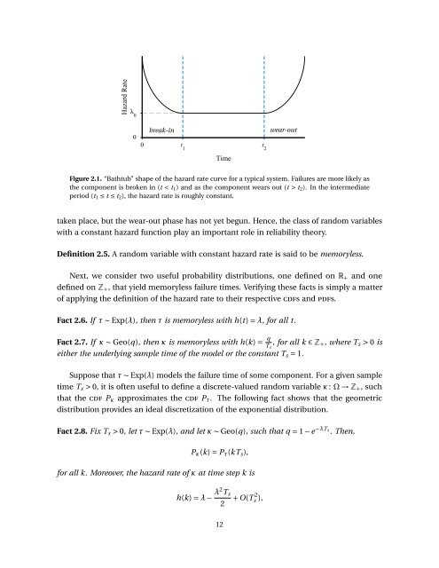
Hazard Rate
λ 0
0
break-in
0 t 1
t 2
Time
wear-out
Figure 2.1. “Bathtub” shape of the hazard rate curve for a typical system. Failures are more likely as
the component is broken in (t < t 1 ) and as the component wears out (t > t 2 ). In the intermediate
period (t 1 ≤ t ≤ t 2 ), the hazard rate is roughly constant.
taken place, but the wear-out phase has not yet begun. Hence, the class of random variables
with a constant hazard function play an important role in reliability theory.
Definition 2.5. A random variable with constant hazard rate is said to be memoryless.
Next, we consider two useful probability distributions, one defined on R + and one
defined on Z + , that yield memoryless failure times. Verifying these facts is simply a matter
of applying the definition of the hazard rate to their respective cdfs and pdfs.
Fact 2.6. If τ ∼ Exp(λ), then τ is memoryless with h(t) = λ, for all t.
Fact 2.7. If κ ∼ Geo(q), then κ is memoryless with h(k) = q T s
, for all k ∈ Z + , where T s > 0 is
either the underlying sample time of the model or the constant T s = 1.
Suppose that τ ∼ Exp(λ) models the failure time of some component. For a given sample
time T s > 0, it is often useful to define a discrete-valued random variable κ: Ω → Z + , such
that the cdf P κ approximates the cdf P τ . The following fact shows that the geometric
distribution provides an ideal discretization of the exponential distribution.
Fact 2.8. Fix T s > 0, let τ ∼ Exp(λ), and let κ ∼ Geo(q), such that q = 1 − e −λT s
. Then,
P κ (k) = P τ (kT s ),
for all k. Moreover, the hazard rate of κ at time step k is
h(k) = λ − λ2 T s
2 +O(T 2 s ),
12