Probabilistic Performance Analysis of Fault Diagnosis Schemes

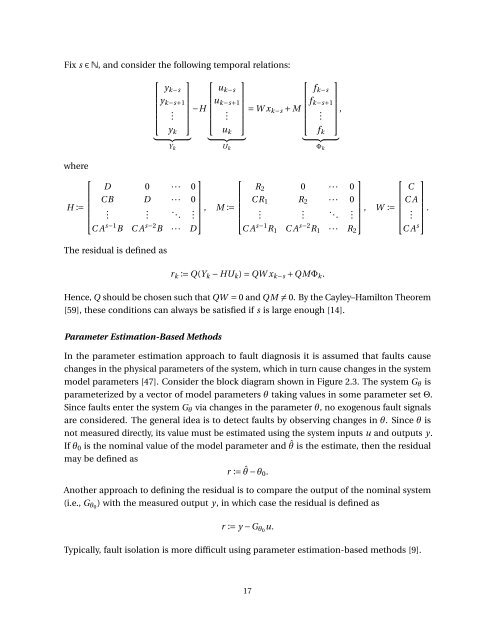
Fix s ∈ N, and consider the following temporal relations:
⎡
⎢
⎣
y k−s
y k−s+1
.
y k
⎤
} {{ }
Y k
⎡
⎥−H
⎢
⎦ ⎣
u k−s
u k−s+1
.
u k
⎤
} {{ }
U k
⎡
f k−s
⎤
f ⎥ = W x k−s + M
k−s+1
⎢ ⎥,
⎦
⎣ . ⎦
f k
} {{ }
Φ k
where
⎡
⎤
D 0 ··· 0
C B D ··· 0
H :=
⎢
.
⎣ . . .. ⎥ . ⎦ ,
C A s−1 B C A s−2 B ··· D
The residual is defined as
⎡
⎤
R 2 0 ··· 0
M := C R 1 R 2 ··· 0
⎢
.
⎣ .
. .. ⎥ . ⎦ ,
C A s−1 R 1 C A s−2 R 1 ··· R 2
⎡ ⎤
C
W := C A
⎢ ⎥
⎣ . ⎦ .
C A s
r k := Q(Y k − HU k ) = QW x k−s +QMΦ k .
Hence, Q should be chosen such that QW = 0 and QM ≠ 0. By the Cayley–Hamilton Theorem
[59], these conditions can always be satisfied if s is large enough [14].
Parameter Estimation-Based Methods
In the parameter estimation approach to fault diagnosis it is assumed that faults cause
changes in the physical parameters of the system, which in turn cause changes in the system
model parameters [47]. Consider the block diagram shown in Figure 2.3. The system G θ is
parameterized by a vector of model parameters θ taking values in some parameter set Θ.
Since faults enter the system G θ via changes in the parameter θ, no exogenous fault signals
are considered. The general idea is to detect faults by observing changes in θ. Since θ is
not measured directly, its value must be estimated using the system inputs u and outputs y.
If θ 0 is the nominal value of the model parameter and ˆθ is the estimate, then the residual
may be defined as
r := ˆθ − θ 0 .
Another approach to defining the residual is to compare the output of the nominal system
(i.e., G θ0 ) with the measured output y, in which case the residual is defined as
r := y −G θ0 u.
Typically, fault isolation is more difficult using parameter estimation-based methods [9].
17