Probabilistic Performance Analysis of Fault Diagnosis Schemes

[ uv1 ]
w 1
f 1
S 1
y 1
[ uv2 ]
w 2
f 2
[ uv3 ]
w 3
f 3
S 2
S 3
y 2
y 3
y 4
mux
y
F
Voting
Scheme
ȳ
−
r
δ
d
[ uv4 ]
w 4
f 4
S 4
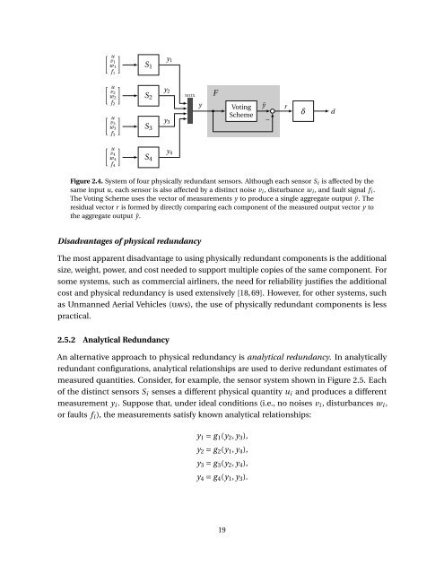
Figure 2.4. System of four physically redundant sensors. Although each sensor S i is affected by the
same input u, each sensor is also affected by a distinct noise v i , disturbance w i , and fault signal f i .
The Voting Scheme uses the vector of measurements y to produce a single aggregate output ȳ. The
residual vector r is formed by directly comparing each component of the measured output vector y to
the aggregate output ȳ.
Disadvantages of physical redundancy
The most apparent disadvantage to using physically redundant components is the additional
size, weight, power, and cost needed to support multiple copies of the same component. For
some systems, such as commercial airliners, the need for reliability justifies the additional
cost and physical redundancy is used extensively [18, 69]. However, for other systems, such
as Unmanned Aerial Vehicles (uavs), the use of physically redundant components is less
practical.
2.5.2 Analytical Redundancy
An alternative approach to physical redundancy is analytical redundancy. In analytically
redundant configurations, analytical relationships are used to derive redundant estimates of
measured quantities. Consider, for example, the sensor system shown in Figure 2.5. Each
of the distinct sensors S i senses a different physical quantity u i and produces a different
measurement y i . Suppose that, under ideal conditions (i.e., no noises v i , disturbances w i ,
or faults f i ), the measurements satisfy known analytical relationships:
y 1 = g 1 (y 2 , y 3 ),
y 2 = g 2 (y 1 , y 4 ),
y 3 = g 3 (y 2 , y 4 ),
y 4 = g 4 (y 1 , y 3 ).
19