Probabilistic Performance Analysis of Fault Diagnosis Schemes
Probabilistic Performance Analysis of Fault Diagnosis Schemes
Probabilistic Performance Analysis of Fault Diagnosis Schemes
Create successful ePaper yourself
Turn your PDF publications into a flip-book with our unique Google optimized e-Paper software.
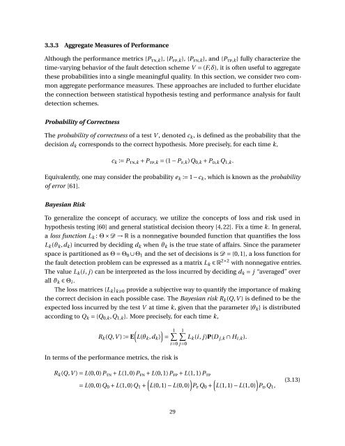
3.3.3 Aggregate Measures <strong>of</strong> <strong>Performance</strong><br />
Although the performance metrics {P tn,k }, {P fp,k }, {P fn,k }, and {P tp,k } fully characterize the<br />
time-varying behavior <strong>of</strong> the fault detection scheme V = (F,δ), it is <strong>of</strong>ten useful to aggregate<br />
these probabilities into a single meaningful quality. In this section, we consider two common<br />
aggregate performance measures. These approaches are included to further elucidate<br />
the connection between statistical hypothesis testing and performance analysis for fault<br />
detection schemes.<br />
Probability <strong>of</strong> Correctness<br />
The probability <strong>of</strong> correctness <strong>of</strong> a test V , denoted c k , is defined as the probability that the<br />
decision d k corresponds to the correct hypothesis. More precisely, for each time k,<br />
c k := P tn,k + P tp,k = (1 − P f,k )Q 0,k + P d,k Q 1,k .<br />
Equivalently, one may consider the probability e k := 1−c k , which is known as the probability<br />
<strong>of</strong> error [61].<br />
Bayesian Risk<br />
To generalize the concept <strong>of</strong> accuracy, we utilize the concepts <strong>of</strong> loss and risk used in<br />
hypothesis testing [60] and general statistical decision theory [4, 22]. Fix a time k. In general,<br />
a loss function L k : Θ × D → R is a nonnegative bounded function that quantifies the loss<br />
L k (ϑ k ,d k ) incurred by deciding d k when ϑ k is the true state <strong>of</strong> affairs. Since the parameter<br />
space is partitioned as Θ = Θ 0 ∪ Θ 1 and the set <strong>of</strong> decisions is D = {0,1}, a loss function for<br />
the fault detection problem can be expressed as a matrix L k ∈ R 2×2 with nonnegative entries.<br />
The value L k (i , j ) can be interpreted as the loss incurred by deciding d k = j “averaged” over<br />
all ϑ k ∈ Θ i .<br />
The loss matrices {L k } k≥0 provide a subjective way to quantify the importance <strong>of</strong> making<br />
the correct decision in each possible case. The Bayesian risk R k (Q,V ) is defined to be the<br />
expected loss incurred by the test V at time k, given that the parameter {θ k } is distributed<br />
according to Q k = {Q 0,k ,Q 1,k }. More precisely, for each time k,<br />
( )<br />
R k (Q,V ) := E L(θ k ,d k )<br />
In terms <strong>of</strong> the performance metrics, the risk is<br />
=<br />
1∑<br />
i=0 j =0<br />
1∑<br />
L k (i , j )P(D j,k ∩ H i ,k ).<br />
R k (Q,V ) = L(0,0)P tn + L(1,0)P fn + L(0,1)P fp + L(1,1)P tp<br />
(<br />
) (<br />
)<br />
= L(0,0)Q 0 + L(1,0)Q 1 + L(0,1) − L(0,0) P f Q 0 + L(1,1) − L(1,0) P d Q 1 ,<br />
(3.13)<br />
29


