WATER & SOIL - These are not the droids you are looking for.

e process of examining the simtrend
was repeated. Adjoining
d a similar trend were combined
together to form a flood frequency region. In this way ll
regions were built up.
In constructing the regions due recognition was taken of
the many factors that would influence the floods in the different
catchments. Attention was given to the climat€, topography
and soils of the catcr,ments, and the aim was to
have catchments with similar flood-producing characteristics
located in the same region. The construction was
guided by maps that showed countrywide climatic and physiographical
patterns, e.g., a Meteorological Service ãvei-
Survey topographical maps.
The ll flood frequency regions that were fîrst decided
upon are shown in Figures 3.6 and 3.7. Four of these regions,
Regions la-ld, were later combined into one (section
3.3.2). The list of stations within each region is given in
Table 3.2.
3.3.2 Development of reglonat flood frequency
cutves
The y values that were used in the regional plots were ob_
tained in the following ma¡ner:
(i) For flood records less than or equal to 35 years in
length, the y values were the exact ones for the unbiased
plotting positions for the EVI distribution and
they were taken from a table in NERC (1975, pp.g2_
3).
(¡i)
0.5 class intervals, and an average e/Q and y value was calculated
from the data points falling within each class. This
averaging process was the same procedure as that used by
NERC (1975) and it produced a smooth trend in the regional
data.
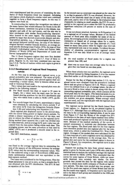
The GEV distribution, namely
In the second case no constraint was placed on the value for
k, so that in general a GEV fit was obtained. However, because
of the relatively small size of many of the data samples
used, and in view of the findings in the evaluation tests
(Appendix A) relating to small samples, the EVI fit was regarded
as the regional curve unless the GEV fit produced a
significant reduction (10 percent or more) in the sum of
squares.
It was not always practical, however, to fit Equation 3.14
to a regional set of average values. Because of the limited
amount of flood peak data available for some of the regions,
the averaging process sometimes produced an unrepresentative
or biased set of average values for a region,
where the average values for low class intervals of y were
based on many data points while for higher class intervals
they represented only one or two points. To reduce the possibility
of obtaining unrepresentative regional curves,
Equation 3.14 was only fitted to a s€t of average values
when:
(l) the total number of flood peaks for a region was
greater than lü); and
(ll) there was no more than one average value for the region
that was based on one data point.
When these criteria were not satisfied, the regional curve
was defined instead by fitting Equation 3.14 in the manner
described ea¡lier to all the plotted data for a region.
Except for the Bay of Plenty (see section 3.3.3), the regional
curves were obtained from the procedures outlined
above and are given in Figures 3.8-3.16. tilhere a regional
curve wÍrs dehned from a set of average values, the plot of
the curve fitted to these values is shown along with the corresponding
regional probability plot, which contains all the
flood peak data for the region. (The historical peaks in a regional
plot are indicated with circles and the corresponding
site numbers are given alongside). Where average valuei
were not used, only the regional plot with the regional curve
superimposed is shown.
The regional curves derived for the North Island West
Coast regions, i.e., Regions la-ld, are plotted together in
Figure 3.17. Although there are differences in the trends of
the data in the corresponding regional plots, it can be seen
from Figure 3.17 that the flrtting of the straight-line EVI
distribution to the data of each region masked these differences
in close agree_
ment.
seeme
the curveS, it
ction between
four regions
for the com-
. Vy'est Coast
region. Averages ofthe pooled data were calculated for the
x=Q/Q
= u*9(l-e-tv¡
k
3t4
24
a :a
=U*oy 323
Support for pooling the data from several regions together
is given by Stevens and Lynn (lg8) who used three
statistical tests to analyse the variation amongst the regional
curves derived by NERC (1975). They concluded that the
curves for some regiôns of Great Britain, while not necessarily
identical, were certainly very similar. On these
grounds they pooled the data for the regions with similar
curves to obtain more stable estimates of floods at high return
periods. The data were pooled into two groups, one
for the fïve south-east regions of Great Britain and one for
the five north-west regions. A frequency curve was then fitted
to the data of each group and extended to the lüXÞyear
return period.
Water & soil technical publication no. 20 (1982)