WATER & SOIL - These are not the droids you are looking for.
WATER & SOIL - These are not the droids you are looking for.
WATER & SOIL - These are not the droids you are looking for.
You also want an ePaper? Increase the reach of your titles
YUMPU automatically turns print PDFs into web optimized ePapers that Google loves.
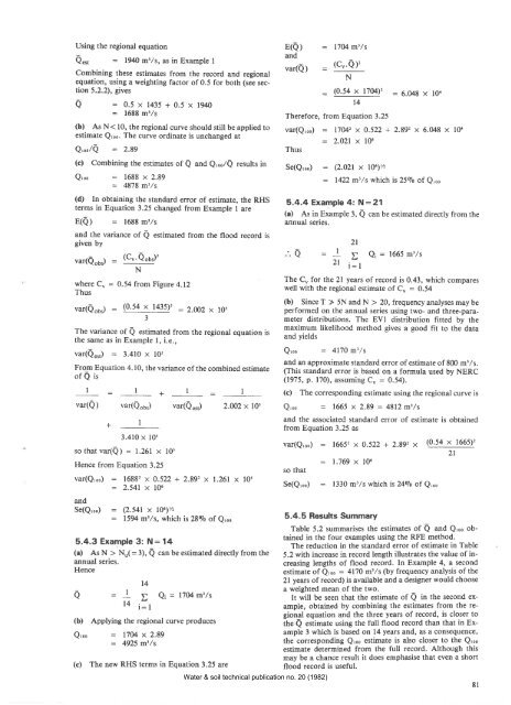
Using <strong>the</strong> regional equation<br />
Qest<br />
1940 m'ls, as in Example I<br />
Combining <strong>the</strong>se estimates from <strong>the</strong> record and regional<br />
equation, using a weighting factor of 0.5 <strong>for</strong> both (see section<br />
5.2.2), gives<br />
a = 0.5x1435+0.5x194O<br />
1688 m',/s<br />
(b) As N< 10, <strong>the</strong> regional curve should still be applied to<br />
estimate Q,oo. The curve ordinate is unchanged at<br />
Q,oolQ : 2.89<br />
(c) Combining <strong>the</strong> estimates of Q and Q,oolQ results in<br />
Q,oo 1688 x 2.89<br />
= 4878 m!/s<br />
(d) In obtaining <strong>the</strong> standard error of estimate, <strong>the</strong> RHS<br />
terms in Equation 3.25 changed from Example I <strong>are</strong><br />
E(Q) = 1688 m3,/s<br />
and <strong>the</strong> variance of Q estimated from <strong>the</strong> flood record is<br />
given by<br />
E(Q)<br />
and<br />
var(Q)<br />
1704 m'ls<br />
(cu.Q)'<br />
N<br />
= (0.54 x 1704)' = 6.048 x 10.<br />
t4<br />
There<strong>for</strong>e, from Equation 3.25<br />
var(Qroo) l1M' x 0.522 + 2.89' x 6.048 x l0'<br />
= 2.021 x 10⁶<br />
Thus<br />
Se(Q'oo) : (2.021 x10⁶)v,<br />
1422 m3/s which is 2590 of Q,oo<br />
5.4.4 Example 4: N:21<br />
(a) As in Example 3, Q can be estimated directly from <strong>the</strong><br />
annual series.<br />
var(Qo6) - (Cn'Qou')'<br />
2t<br />
N<br />
i]r<br />
where C" :<br />
The Cn <strong>for</strong> <strong>the</strong> 0.54 from<br />
2l years of record is 0.43, which comp<strong>are</strong>s<br />
Figure 4.12<br />
well with <strong>the</strong> regional estimate of C" : 9.54<br />
Thus<br />
var(Qo6) : (0.54 x<br />
(b) Since T ) 5N and N > 20, frequency analyses may be<br />
1435)' : 2.002 x l0'<br />
per<strong>for</strong>med on <strong>the</strong> annual series using two- and three-parameter<br />
distributions. The EVI distribution fitted by <strong>the</strong><br />
3<br />
The variance<br />
maximum<br />
of<br />
likelihood method gives<br />
Q estimated from<br />
a good fit to <strong>the</strong> data<br />
<strong>the</strong> regional equation is<br />
<strong>the</strong><br />
and yields<br />
same as in Example l, i.e.,<br />
var(QesJ = 3.410x10⁵<br />
Q'oo<br />
: 4l7O m'/s<br />
and an approximate standard error of estimate of 800 m',/s.<br />
From Equation 4.10, <strong>the</strong> variance of <strong>the</strong> combined estimate (This<br />
of Q is<br />
standard error is based on a <strong>for</strong>mula used by NERC<br />
(1975, p. 170), assuming Cu : 0.54).<br />
l:l+l<br />
(c) The corresponding estimate using <strong>the</strong> regional curve is<br />
var(Q) var(Qo') var(Q.r¡) 2.002 x l0r Q,oo 1665x2.89:4812m3/s<br />
and <strong>the</strong> associated standard error of estimate is obtained<br />
+<br />
from Equation 3.25 as<br />
3.410 x l0r<br />
var(Q,oo) 1665' x 0.522 + 2.8g'z x<br />
(0'54 x 1665)'z<br />
so that var(Q) = 1.261 x 10⁵<br />
2l<br />
Hence from Equation<br />
1.769 x loó<br />
3.25<br />
so that<br />
var(Qroo) 1688' 0.522 + 2.89'? x 1.261 x 10⁵<br />
: 2.541 x Se(Q'oo) 1330 m3,/s which is 2490 of<br />
106<br />
Q,oo<br />
and<br />
Se(Q,oo) = (2.541 x l0ó)/z<br />
1594 m!/s, which is 2890 of Q,oo<br />
5.4.5 Results Summary<br />
Table 5.2 summarises <strong>the</strong> estimates of Q and Q'oo obtained<br />
in <strong>the</strong> four examples using <strong>the</strong> RFE method.<br />
5.4.3 Example 3: N: 14<br />
The reduction in <strong>the</strong> standard error of estimate in Table<br />
(a) As N > N"( = 3), Q can be estimated directly from <strong>the</strong> 5.2 with increase in record length illustrates <strong>the</strong> value of increasing<br />
lengths of flood record. In Example 4, a second<br />
annual series.<br />
Hence<br />
estimate of Q,oo : 4l7O m'ls (by frequency analysis of <strong>the</strong><br />
l4<br />
2l years ofrecord) is available and a designer would choose<br />
a = I a weighted mean of <strong>the</strong> two.<br />
I ei =1704m',/s<br />
It will be seen that <strong>the</strong> estimate of Q in <strong>the</strong> second example,<br />
obtained by combining <strong>the</strong> estimates from <strong>the</strong> re-<br />
14 i-: I<br />
gional equation and <strong>the</strong> three years of record, is closer to<br />
(b) Applying <strong>the</strong> regional curve produces<br />
<strong>the</strong> Q estimate using <strong>the</strong> full flood record than that in Example<br />
3 which is based on 14 years and, as a consequence,<br />
Q'oo :1704 x2.89<br />
= 4925 m3/s<br />
<strong>the</strong> corresponding Q,oo estimate is also closer to <strong>the</strong> Qroo<br />
estimate determined from <strong>the</strong> full record. Although this<br />
may be a chance result it does emphasise that even a short<br />
(c) The new RHS terms in Equation 3.25 <strong>are</strong><br />
flood record is useful.<br />
Water & soil technical publication no. 20 (1982)<br />
81<br />
a<br />
2t<br />
= I )- Qi:1665m'/s


