The Winton M. Blount Postal History Symposia - Smithsonian ...

More documents

Recommendations

Info

3 2 • s m i t h s o n i a n c o n t r i b u t i o n s t o h i s t o ry a n d t e c h n o l o g ypublished in the statutes relating compensation to totalpostal income, it should be possible to derive total postalincome from the compensation data. For example, in 1859the Concord NH postmaster received $1,783 (rounded tothe nearest dollar) in compensation. But for the year 1859the OR reports not only the compensation but also thenet income. Adding the two together produces total postalincome of $5,424. 19 If compensation were based only onpostal income, a calculation of the 1859 Concord post officeincome using the compensation rates in effect at thetime should result in a figure of approximately $5425.This calculation actually yields a figure of $7,553, a differenceof $2,129, or thirty-nine percent (Table 1).This calculated figure is higher than the actual incomebecause postmaster compensation included monies forthings other than postal income such as box rents, extrapay for delivery of late mails, delivery of newspapers, andthe like. One would expect that the discrepancy betweenthe actual reported income and estimated income would bein the positive direction. Further, the discrepancy should belarger for larger post offices where the postmaster wouldhave greater opportunities for earning additional compensationnot directly related to the amount of money his officereceived. To test this hypothesis and to get an ideaof how generally reflective of true total postal income thereported compensation figures were, a total of twenty-fiveNew Hampshire post offices varying in size were selectedfrom the 1859 OR. For each office, the compensationdue based on the reported compensation plus net incomefigure was calculated. The difference was then expressedas a percentage with positive percentages indicating thereported compensation was greater than the calculatedcompensation. The average difference was twelve percentwith a standard deviation of twenty-two. Of the twentyfiveoffices, nineteen had positive differences and six hadnegative differences.Positive differences are fairly easy to explain. Postmastercompensation included monies for things otherthan postage paid at the office. Depending on the specificcompensation rules in effect, these included extra compensationfor such things as receipt of newspapers, post officebox rents, onward routing of letters, receipts of mails aftera certain time at night. These extra sources of compensationa postmaster earned would be more likely to occur atthe larger post offices. This supposition is supported bythe significant correlation of reported compensation withthe percentage difference between reported and calculatedcompensation and is significant with r = + .40 (p < .047).The negative differences may have been due to finesfor various infractions, but additional research will beneeded to investigate the rules for such fines and the characteristicsof post offices with negative differences.Two other variables had some effect on compensation.Postmasters received extra compensation (usually tenpercent) of the first compensation increment if they had toopen their office at late hours to receive or dispatch themail. Postmasters at “distributing offices” which receivedand then sorted mail bound for other offices also receivedextra compensation. There were no distributing offices inNew Hampshire after 1842. In earlier years only Hanover(until 1837 or 1838), Portsmouth (until 1837 or 1838)and Walpole (until at least 1831) were distributing officesin the state.TABLE 1. Calculation of estimated income for Concord, NH1859.Actual Compensation Net Sum$1783 $3641 $5424Calculation:income CompensationRange Amount Percent Compensation Remainder$1783$0–$100 $100 60% $60 $1723$100–$400 $300 50% $150 $1573$400–$2400 $2000 40% $800 $773$2400+ $5153 15% $773 $0Sum $7553 $1783Population EffectsIn the previous section the general validity of calculatingestimated post office income from the published postmastercompensation data was established. This being thecase, it is appropriate to investigate further the factors thatcorrelate with the estimated income variable. An obviouscandidate is population. A simple prediction is that as thepopulation of a town or city increases, so will the amountof business its post office does, resulting in a higher postalincome for that town. There are two ways to examine therelationship between population and estimated income.The first is to examine the relationship for each censusyear for which data is available. Here this means the decennialcensus years of 1820 to 1910. The year 1880 isnot included in the percent analysis as the law in effect
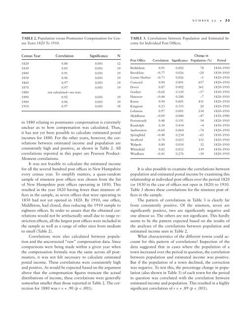
n u m b e r 5 5 • 3 3TABLE 2. Population versus Postmaster Compensation for CensusYears 1820 To 1910.TABLE 3. Correlations between Population and Estimated Incomefor Individual Post Offices.Census Year Correlation Significance N1820 0.88 0.001 121830 0.85 0.001 191840 0.91 0.001 191850 0.96 0.001 191860 0.97 0.001 191870 0.97 0.001 191880 not calculated—see text.1890 0.92 0.001 191900 0.96 0.001 191910 0.97 0.001 18in 1880 relating to postmaster compensation is extremelyunclear as to how compensation was calculated. Thus,it has not yet been possible to calculate estimated postalincomes for 1880. For the other years, however, the correlationsbetween estimated income and population areconsistently high and positive, as shown in Table 2. Allcorrelations reported in this paper are Pearson Product-Moment correlations.It was not feasible to calculate the estimated incomefor all the several hundred post offices in New Hampshireevery census year. To simplify matters, a quasi-randomsample of nineteen post offices was chosen from the listof New Hampshire post offices operating in 1850. Thisresulted in the year 1820 having fewer than nineteen officesin the sample, as seven offices that were operating in1850 had not yet opened in 1820. By 1910, one office,Middleton, had closed, thus reducing the 1910 sample toeighteen offices. In order to assure that the obtained correlationswould not be artifactually small due to range restrictioneffects, all the largest post offices were included inthe sample as well as a range of other sizes from mediumto small (Table 2).Correlations were also calculated between populationand the uncorrected “raw” compensation data. Sincecomparisons were being made within a given year whenthe compensation formula was the same across all postmasters,it was not felt necessary to calculate estimatedpostal income. These correlations were consistently highand positive. As would be expected based on the argumentabove that the compensation figures truncate the actualdistributions of income, these correlations were generallysomewhat smaller than those reported in Table 2. The correctionfor 1880 was r = + .90 (p < .001).Change inPost Office Correlation Significance Population (%) PeriodBethlehem 0.91 0.002 78 1830–1910Brookline –0.77 0.026 –20 1830–1910Center Harbor –0.73 0.026 –1 1820–1910Concord 0.90 0.001 657 1820–1910Dover 0.87 0.002 361 1820–1910Goshen –0.60 0.120 –57 1830–1910Hanover –0.44 0.240 –7 1820–1910Keene 0.94 0.001 431 1820–1910Kingston 0.23 0.555 20 1820–1910Lebanon 0.97 0.001 234 1820–1910Middleton –0.09 0.840 –47 1830–1900Portsmouth 0.48 0.191 54 1820–1910Randolph 0.34 0.414 –4 1830–1910Sanbornton –0.64 0.064 –74 1820–1910Springfield –0.48 0.234 –65 1830–1910Strafford 0.74 0.023 152 1820–1910Walpole 0.80 0.010 32 1820–1910Whitefield 0.82 0.012 139 1830–1910Windham –0.41 0.276 –34 1820–1910It is also possible to examine the correlations betweenpopulation and estimated postal income by examining thisrelationship at individual post offices over the period 1820(or 1830 in the case of offices not open in 1820) to 1910.Table 3 shows these correlations for the nineteen post officesin the sample.The pattern of correlations in Table 3 is clearly farfrom consistently positive. Of the nineteen, seven aresignificantly positive, two are significantly negative andone almost so. The others are not significant. This hardlyseems to be the pattern expected based on the results ofthe analyses of the correlations between population andestimated income seen in Table 2.What characteristics of the different towns could accountfor this pattern of correlations? Inspection of thedata suggested that in cases where the population of atown increased over the period in question, the correlationbetween population and estimated income was positive.But if the population of a town declined, the correctionwas negative. To test this, the percentage change in population(also shown in Table 3) of each town for the periodin question was correlated with the correlation betweenestimated income and population. This resulted in a highlysignificant correlation of r = + .89 (p < .001).
Page 1 and 2: Smithsonian InstitutionScholarly Pr
Page 3 and 4: smithsonian contributions to histor
Page 5: ContentsLETTER FROM THE DIRECTOR OF
Page 9: AcknowledgmentsThe symposium would
Page 12 and 13: 2 • s m i t h s o n i a n c o n t
Page 20 and 21: 1 0 • s m i t h s o n i a n c o n
Page 25 and 26: “Little Colored Bits of Paper”C
Page 27 and 28: n u m b e r 5 5 • 1 7as something
Page 29 and 30: n u m b e r 5 5 • 1 9protest came
Page 31 and 32: n u m b e r 5 5 • 2 1nals I revie
Page 33 and 34: WWI Philatelic Censuses of East Afr
Page 35 and 36: n u m b e r 5 5 • 2 5Table 1. GEA
Page 37 and 38: n u m b e r 5 5 • 2 7Figure 5. MA
Page 39 and 40: Explorations in the Official Regist
Page 41: n u m b e r 5 5 • 3 1receipts. De
Page 45 and 46: n u m b e r 5 5 • 3 5different ge
Page 47: Introduction to the Second Symposiu
Page 59 and 60: “Food Will Win the War”: Motor
Page 61 and 62: n u m b e r 5 5 • 5 1business tha
Page 63 and 64: n u m b e r 5 5 • 5 3support for
Page 65 and 66: n u m b e r 5 5 • 5 53. “Postal
Page 67: n u m b e r 5 5 • 5 7“Farmers W
Page 81 and 82: Picking Up the Pieces: The Aftermat
Page 83 and 84: n u m b e r 5 5 • 7 3and U.S. adm
Page 85 and 86: n u m b e r 5 5 • 7 5September, 1
Page 87 and 88: n u m b e r 5 5 • 7 7Figure 9. Th
Page 89: n u m b e r 5 5 • 7 9“B.C.O.F.
Page 92 and 93:
8 2 • s m i t h s o n i a n c o n
Page 94 and 95:
Page 96 and 97:
Page 98 and 99:
Page 101:
Introduction to the Fourth Symposiu
Page 104 and 105:
Page 106 and 107:
Page 108 and 109:
Page 110 and 111:
1 0 0 • s m i t h s o n i a n c o
Page 112 and 113:
1 0 2 • s m i t h s o n i a n c o
Page 114 and 115:
1 0 4 • s m i t h s o n i a n c o
Page 116 and 117:
1 0 6 • s m i t h s o n i a n c o
Page 118 and 119:
1 0 8 • s m i t h s o n i a n c o
Page 120 and 121:
1 1 0 • s m i t h s o n i a n c o
Page 122 and 123:
1 1 2 • s m i t h s o n i a n c o
Page 124 and 125:
1 1 4 • s m i t h s o n i a n c o
Page 126 and 127:
1 1 6 • s m i t h s o n i a n c o
Page 128 and 129:
1 1 8 • s m i t h s o n i a n c o
Page 131 and 132:
“Why Is a Raven Like a Writing De
Page 133 and 134:
n u m b e r 5 5 • 1 2 3and prepai
Page 135 and 136:
n u m b e r 5 5 • 1 2 5Figure 3.
Page 137 and 138:
n u m b e r 5 5 • 1 2 7Figure 5.
Page 139 and 140:
n u m b e r 5 5 • 1 2 9A Final No
Page 141 and 142:
America’s First Carrier Service:T
Page 143 and 144:
n u m b e r 5 5 • 1 3 3Figure 3.
Page 145 and 146:
n u m b e r 5 5 • 1 3 5The glazed
Page 147 and 148:
n u m b e r 5 5 • 1 3 7Intercity
Page 149 and 150:
n u m b e r 5 5 • 1 3 9The End of
Page 151 and 152:
The U.S. 1847 Issue:Stamps That Cha
Page 153 and 154:
n u m b e r 5 5 • 1 4 3the positi
Page 155 and 156:
n u m b e r 5 5 • 1 4 5stamps as
Page 157 and 158:
From the Pulpit to the Post: Anti-
Page 159 and 160:
n u m b e r 5 5 • 1 4 9The allege
Page 161 and 162:
n u m b e r 5 5 • 1 5 1Individual
Page 163:
n u m b e r 5 5 • 1 5 337. Archiv
Page 166 and 167:
1 5 6 • s m i t h s o n i a n c o
Page 168 and 169:
1 5 8 • s m i t h s o n i a n c o
Page 170 and 171:
1 6 0 • s m i t h s o n i a n c o
Page 172 and 173:
1 6 2 • s m i t h s o n i a n c o
Page 174 and 175:
1 6 4 • s m i t h s o n i a n c o
Page 176 and 177:
1 6 6 • s m i t h s o n i a n c o
show all

The Winton M. Blount Postal History Symposia - Smithsonian ...

Create successful ePaper yourself

Delete template?

Save as template?