coulomb excitation data analysis codes; gosia 2007 - Physics and ...

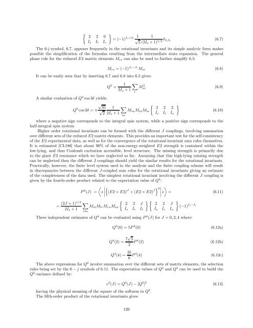
½ ¾2 2 0=(−1) 1 1I s I t I Is+Ir √r 5 (2I s +1) δ 1/2 I s I t(6.7)The 6-j symbol, 6.7, appears frequently in the rotational invariants and its simple analytic form makespossible the simplification of the formulas resulting from the intermediate state expansion. The generalphase rule for the reduced E2 matrix elements M rs can also be used to further simplify 6.5:It can be easily seen that by inserting 6.7 and 6.8 into 6.5 gives:M rs =(−1) Js−Jr M sr (6.8)Q 2 =12I s +1tuXMsr 2 (6.9)A similar evaluation of Q 3 cos 3δ yields:√35Q 3 1 X½ ¾2 2 2cos 3δ = ∓ √ M su M ut M ts2 2I s +1I s I t I ur(6.10)where a negative sign corresponds to the integral spin system, while a positive sign corresponds to thehalf-integral spin system.Higher order rotational invariants can be formed with the different J couplings, involving summationover different sets of the reduced E2 matrix elements. This provides an important test for the self-consistencyof the E2 experimental data, as well as for the convergence of the rotational-invariant sum rules themselves.It is estimated [CL186] that about 90% of the non-energy-weighted E2 strength is contained within thelow-lying, and thus Coulomb excitation accessible, level structure. The missing strength is primarily dueto the giant E2 resonance which we have neglected so far. Assuming that this high-lying missing strengthcan be neglected then the different J couplings should yield the similar results for the rotational invariants.Practically, however, the finite level system used in the analysis and the finite coupling scheme will resultin discrepancies between the different J-coupled sum rules for the rotational invariants giving an estimateof the completeness of the data used. The simplest rotational invariant involving the different J coupling isgiven by the fourth-order product related to the expectation value of Q 4 :¿nP 4 (J) = s¯ (E2 × E2) J × (E2 × E2) Jo À0¯¯¯¯ s = (6.11)=(2J +1)1/22I s +1Xrtu½ ¾½ ¾2 2 J 2 2 JM st M tr M ru M us (−1)I s I r I t I s I r I Is−IruThree independent estimates of Q 4 can be evaluated using P 4 (J) for J =0, 2, 4 where:Q 4 (0) = 5P 4 (0)(6.12a)Q 4 (2) = 7√ 52 P 4 (2) (6.12b)Q 4 (4) = 35 6 P 4 (4)(6.12c)The above expressions for Q 4 involve summation over the different sets of matrix elements, the selectionrules being set by the 6 − j symbols of 6.11. The expectation values of Q 2 and Q 4 canbeusedtobuildtheQ 2 -variance defined by:having the physical meaning of the square of the softness in Q 2 .The fifth-order product of the rotational invariants givesv 2 (J) =Q 4 (J) − [Q 2 ] 2 (6.13)120