coulomb excitation data analysis codes; gosia 2007 - Physics and ...

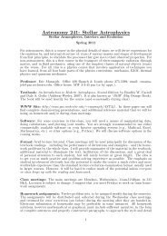
(1.6 MeV)1.1 MeV0.75 MeV0.4 MeV0.08+ Level “5” – Unobserved “buffer state”6+ Level “4”4+ Level “3”2+ Level “2”0+ Level “1”Figure 13: Fictitious level scheme of the nucleus to be investigated in the toyfit.tar demo. Levels are labeledwith their energy, spin, and the index used in the Gosia inputs. Arrows represent the E2 matrix elementsentered in the Gosia inputs with the consistent phase convention as shown. Three E2 diagonal moments areincluded. The 8 + is a "buffer state" required for accurate calculation of the 6 + state yields. See section 5.13.35,70,240,70,4,0,0,0,360,1,1defines the “un-investigated” nucleus (Z=35, A=70), the mean beam energy in the target (240MeV), themean laboratory scattering angle (70 degrees polar). The remaining fields define accuracy parameters for thepoint calculations, symmetry of the detector (azimuthal symmetry in this case), normal or inverse kinematics(irrelevant here) and normalization to other experiments (also irrelevant here).The CONT block is used to set a number of options including fixing/freeing of matrix elements, outputoptions, the use of PIN diodes as particle detectors, etc.Note that a blank line is required after the flag END,The 4 th option in this input is OP,YIEL, whichallowstheusertodefine the gamma-ray detectorlocations, internal conversion coefficients, normalization constants between experiments (irrelevant in thiscase), tabulated data (branching ratios, lifetimes, mixing ratios and measured matrix elements), etc. Theuser is referred to section 5.30 (OP,YIEL) for a detailed description. The following are of particular interestto the first time user. (Note that the line numbers will vary with the complexity of the experimental setup.)Lines 2 - 7: These are the internal conversion data entered by the user from tables, such as those fromBRICC.Lines 9 - 11: This declares that a Ge detector of type “1” in the detector file (“det.gdt” in this case) ispositioned at a polar angle of 45 degrees and an azimuthal angle (arbitrary 0) of 90 degrees. Only one Gedetector is defined in this experiment!NTAP is set to 0, which tells Gosia that no experimental yields are to be read from disk. Obviously,experimental data are not used to simulate yields.The final option used is OP,INTG, which integrates the point calculations over the particle scatteringangles and the beam energy range as the projectile traverses the target. If azimuthally symmetric particledetectors are used, the target is “investigated” and the beam particle is detected, as in the present case, theinput is relatively simple with the first three lines corresponding to experiment 1. Line 1,5,5,230,250,60,80indicates that 5 equally-spaced energy meshpoints and 5 polar scattering angle meshpoints will be providedby the user. The energy range as the beam traverses the target is 250–230 MeV, and the particle detectorcovers the laboratory scattering angles 60–80 degrees. In the present version of Gosia, the energy rangemust be calculated by the user from tabulated stopping power data. Line 2 gives the energy meshpoints,and line 3 gives the scattering angle meshpoints, both of which must exceed the integration range.Lines 4 - 6 give stopping power data for the beam and target combination. (In the present case, thestopping power is about 32 MeV per mg/cm 2 , and the energy range in the target is 20 MeV, so the targetthickness is about 2/3 mg/cm 2 .)Line 7 gives the number of subdivisions in energy and scattering angle to be used for the fast interpolation157