coulomb excitation data analysis codes; gosia 2007 - Physics and ...

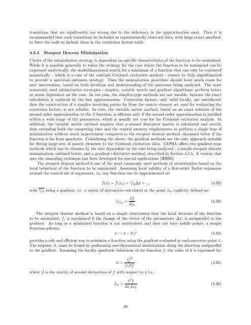
transitions that are significantly too strong due to the deficiency in the approximation used. Then it isrecommended that such transitions be included as experimentally observed data, with large errors ascribed,to force the code to include them in the correction factors table.4.5.4 Steepest Descent MinimizationChoice of the minimization strategy is dependent on specific characteristics of the function to be minimized.While it is possible generally to tailor the strategy for the case where the function to be minimized can beexpressed analytically, the multidimensional search for a minimum of a function that can only be evaluatednumerically - which is a case of the multiple Coulomb excitation analysis - cannot be fully algorithmizedto provide a universal optimum strategy. Thus the minimization procedure should leave much room foruser intervention, based on both intuition and understanding of the processes being analyzed. The mostcommonly used minimization strategies - simplex, variable metric and gradient algorithms- perform betteror worse dependent on the case. In our case, the simplex-type methods are not useable, because the exactcalculation is replaced by the fast approximation. Correction factors, only valid locally, are introduced,thus the construction of a simplex involving points far from the matrix element set used for evaluating thecorrection factors, is not reliable. In turn, the variable metric method, based on an exact solution of thesecond-order approximation to the S function, is efficient only if the second-order approximation is justifiedwithin a wide range of the parameters, which is usually not true for the Coulomb excitation analysis. Inaddition, the variable metric method requires that a second derivative matrix is calculated and stored,thus extending both the computing time and the central memory requirements to perform a single step ofminimization without much improvement compared to the steepest descent method, discussed below if thefunction is far from quadratic. Considering the above, the gradient methods are the only approach suitablefor fitting large sets of matrix elements to the Coulomb excitation data. GOSIA offers two gradient-typemethods which can be choosen by the user dependent on the case being analyzed - a simple steepest descentminimization, outlined below, and a gradient+derivative method, described in Section 4.5.5. A version thatuses the annealing technique has been developed for special applications [IBB95]The steepest descent method is one of the most commonly used methods of minimization based on thelocal behaviour of the function to be minimized. Assuming local validity of a first-order Taylor expansionaround the central set of arguments, ¯x 0 , any function can be approximated as:f(¯x) =f(¯x 0 )+ ¯5 0 ∆¯x + ... (4.32)with 5 0 being a gradient, i.e. a vector of derivatives calculated at the point ¯x 0 , explictly defined as:¯5 0,i = δfδx i(4.33)The steepest descent method is based on a simple observation that the local decrease of the functionto be minimized, f, is maximized if the change of the vector of the parameters, ∆¯x, is antiparallel to thegradient. As long as a minimized function is not multivalued and does not have saddle points, a simpleiteration scheme:¯x → ¯x − h ¯5 (4.34)provides a safe and efficient way to minimize a function using the gradient evaluated at each succesive point ¯x.The stepsize, h, must be found by performing one-dimensional minimization along the direction antiparallelto the gradient. Assuming the locally quadratic behaviour of the function f, thevalueofh is expressed by:h = ¯5 2¯5J ¯5(4.35)where J is the matrix of second derivatives of f with respect to ¯x i.e.:J ik =δ2 fδx i δx k(4.36)46