Welcome to Adams/Solver Subroutines - Kxcad.net

F(M 1 (q), M 2 (q), ..., M N (q))
Welcome to Adams/Solver Subroutines
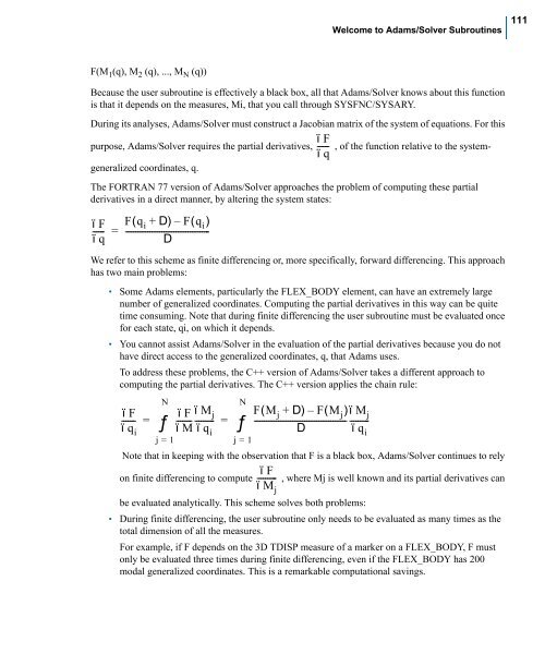
Because the user subroutine is effectively a black box, all that Adams/Solver knows about this function
is that it depends on the measures, Mi, that you call through SYSFNC/SYSARY.
During its analyses, Adams/Solver must construct a Jacobian matrix of the system of equations. For this
purpose, Adams/Solver requires the partial derivatives, , of the function relative to the system-
generalized coordinates, q.
The FORTRAN 77 version of Adams/Solver approaches the problem of computing these partial
derivatives in a direct manner, by altering the system states:
∂ F
-----
∂ q
F( qi + ∆)
– F( qi) = -----------------------------------------
∆
We refer to this scheme as finite differencing or, more specifically, forward differencing. This approach
has two main problems:
• Some Adams elements, particularly the FLEX_BODY element, can have an extremely large
number of generalized coordinates. Computing the partial derivatives in this way can be quite
time consuming. Note that during finite differencing the user subroutine must be evaluated once
for each state, qi, on which it depends.
• You cannot assist Adams/Solver in the evaluation of the partial derivatives because you do not
have direct access to the generalized coordinates, q, that Adams uses.
To address these problems, the C++ version of Adams/Solver takes a different approach to
computing the partial derivatives. The C++ version applies the chain rule:
∂ F
-------
∂ qi N
∂ F
-------
∂ M
∂ Mj = ∑ --------- =
∂ qi j = 1
N
∑
j = 1
Note that in keeping with the observation that F is a black box, Adams/Solver continues to rely
on finite differencing to compute , where Mj is well known and its partial derivatives can
be evaluated analytically. This scheme solves both problems:
• During finite differencing, the user subroutine only needs to be evaluated as many times as the
total dimension of all the measures.
For example, if F depends on the 3D TDISP measure of a marker on a FLEX_BODY, F must
only be evaluated three times during finite differencing, even if the FLEX_BODY has 200
modal generalized coordinates. This is a remarkable computational savings.
∂ F
-----
∂ q
F( Mj + ∆)
– F( Mj) ----------------------------------------------
∆
∂ Mj ---------
∂ qi ∂ F
---------
∂ Mj 111